22 Examples of Recursive Functions in Python
Posted by Al Sweigart in misc

This blog post contains information from Al Sweigart's next book, The Recursive Book of Recurson from No Starch Press. The book will be released in June 2022. You can use the discount code PREORDERRECURSION to get 30% off your preorder, and receive the ebook free when you buy a print book. This book will also be freely available under a Creative Commons license on the Invent with Python website. Al Sweigart also gave a conference talk on recursion at North Bay Python 2018 titled, Recursion for Beginners: A Beginner's Guide to Recursion.
Here are 22 actual, runnable Python code for several recursive functions, written in a style to be understandable by beginners and produce debuggable output.
These are not code snippets; they are complete, runnable Python programs. The source code has been put inside a text field to make scrolling through this blog post easier. You can click on the text field, select all by pressing Ctrl-A, then copy the code to the clipboard by pressing Ctrl-C. Once on the clipboard, you can paste it into your editor or IDE. There are also download links for each of the programs as well.
These recursive functions are also designed to produce helpful, teachable output. Some of the functions have an indent parameter to aid in this output and isn't a part of the recursive algorithm itself.
Ackermann
The Ackermann function is named after its discoverer, Wilhelm Ackermann. Ackermann, a student of mathematician David Hilbert (creator of the Hilbert curve fractal), published his function in 1928. Mathematicians Rózsa Péter and Raphael Robinson later developed the version of the function featured in this section. While the Ackermann function has some application in advanced mathematics, it is mostly known for being an example of a highly recursive function. Even slight increases to its two integer arguments cause a large increase in the number of recursive calls it makes.
Computerphile YouTube channel has a video on it titled, "The Most Difficult Program to Compute?"
The output of this program looks like this:
Binary Search
Binary search is a technique for locating a target item in a sorted list by re-peatedly determining which half of the list the item is in. The most impartial way to search the bookshelf is to start with a book in the middle, then ascertain if the target book you’re looking for is in the left half or the right half.
You can then repeat this process: look at the book in the middle of your chosen half, and determine if your target book is in the left-side quarter or the right-side quarter. You can do this until you either find the book or find the place where the book should be but isn’t and declare that the book doesn’t exist on the shelf.
The output of this program looks like this:
Combinations
Given a set of items, we can return a set of every combination of those items. For example, given a set of four letters, ABCD, the k-combinations are:
- The 0-combinations and 4-combinations have one combination: the empty string and ABCD respectively.
- The 1-combinations and 3-combinations have four combinations: A, B, C, D and ABC, ABD, ACD, BCD, respectively.
- The 2-combinations have the most combinations at six combinations: AB, AC, AD, BC, BD, and CD.
The output of this program looks like this:
Count Down and Up
This function is a demonstration of a simple recursive function and shows the order that code runs before and after the recursive call.
The output of this program looks like this:
Drunk Sierpinski Triangle
Download drunkSierpinskiTriangle.py
This program uses the turtle module to draw a sierpinski triangle fractal, except with slight errors to give the fractal a distorted look.
The output of this program looks like this:

Eight Queens
The eight queens puzzle is how to find an arrangement of eight chess queens on a board such that they cannot attack each other. This recursive program finds every possible solution on an 8 x 8 chess board.
The output of this program looks like this:
Exponentiation
Download exponentWithPowerRule.py
Calculating exponents such as 2^5 (or 2 x 2 x 2 x 2 x 2) can be done without using the ** operator by doing repeat multiplications. However, there's a shortcut in that 2^(m * 2) == 2^m * 2^m. You can use this trick to perform a^m in less than m multiplications.
The output of this program looks like this:
Factorial
Download factorialByRecursion.py
The factorial of 4 is 4 × 3 × 2 × 1 and the factorial of 5 is 5 × 4 × 3 × 2 × 1. So you could say that 5! = 5 × 4!. This is recursive because the definition of the factorial of 5 (or any number n) includes the definition of the factorial of 4 (the number n – 1). In turn, 4! = 4 × 3!, and so on, until you must calculate 1!, the base case, which is simply 1.
The output of this program looks like this:
Fibonacci
Download fibonacciByRecursion.py
The Fibonacci sequence is another classic example for introducing recursion. Mathematically, the Fibonacci sequence of integers begins with the numbers 1 and 1 (or sometimes, 0 and 1). The next number in the sequence is the sum of the previous two numbers. This creates the sequence 1, 1, 2, 3, 5, 8, 13, 21, 34, 55, 89, 144, and so on, forever.
There is a recursive property to calculating Fibonacci numbers. For example, if you want to calculate the 10th Fibonacci number, you add the 9th and 8th Fibonacci numbers together. To calculate those Fibonacci numbers, you add the 8th and 7th, then the 7th and 6th Fibonacci numbers. There’s going to be a lot of repeat calculations: notice that adding the 9th and 8th Fibonacci number involves calculating the 8th Fibonacci number again. You would continue this recursion until you reach the base case of the 1st or 2nd Fibonacci numbers, which are always 1.
The output of this program looks like this:
Floodfill
The output of this program looks like this:
GCD, Greatest Common Denominator
Factors are the numbers that are multiplied to produce a particular number. Consider 4 × 6 = 24. In this equation, 4 and 6 are factors of 24. Because a number’s factors can also be used to divide that number without leaving a remainder, factors are also called divisors.
The factors of 24 are 1, 2, 3, 4, 6, 8, 12, and 24. The factors of 30 are 1, 2, 3, 5, 6, 10, 15, and 30. Note that any number will always have 1 and itself as its factors because 1 times a number is equal to that number. Notice too that the list of factors for 24 and 30 have 1, 2, 3, and 6 in common. The greatest of these common factors is 6, so 6 is the greatest common factor, more commonly known as the greatest common divisor (GCD), of 24 and 30.
Euclid, a mathematician who lived 2000 years ago, came up with a short algorithm for finding the GCD of two numbers using modular arithmetic. His algorithm can be implemented with recursion:
The output of this program looks like this:
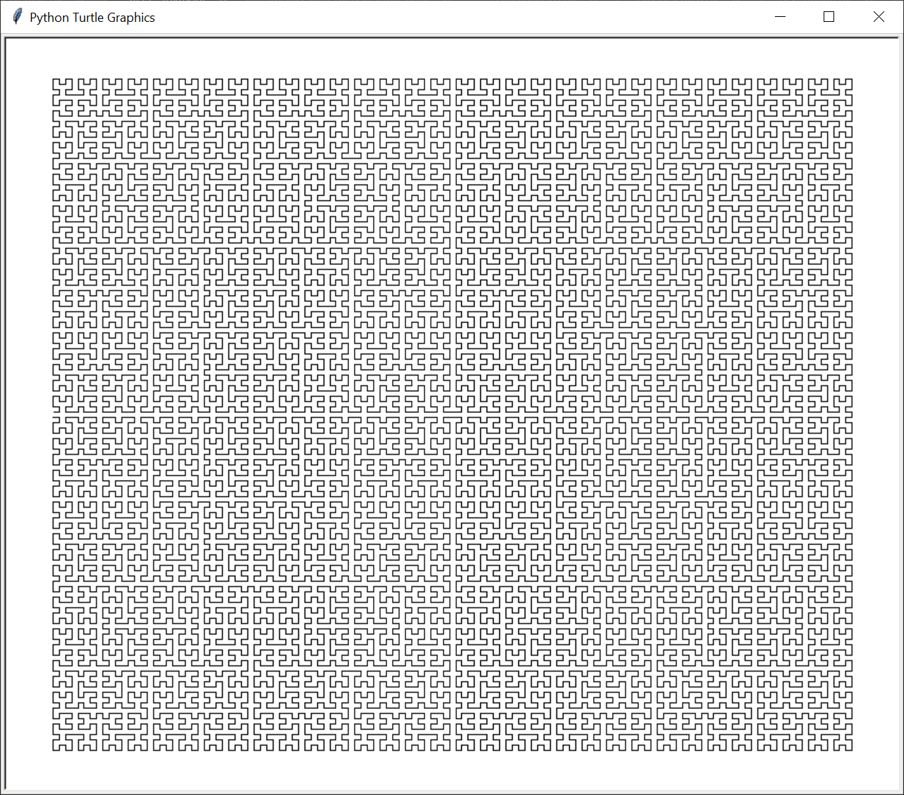
Hilbert Curve Fractal
A space-filling curve is a one-dimensional line that curves around until it completely fills a two-dimensional space without crossing over itself. German mathematician David Hilbert described his space-filling Hilbert curve in 1891.
The output of this program looks like this:
Karatsuba Multiplication
Download karatsubaMultiplication.py
Karatsuba multiplication is a fast, recursive algorithm discovered by Anatoly Karatsuba in 1960 that can multiply integers using addition, subtraction, and a pre-computed multiplication table of all products from single-digit numbers.
The output of this program looks like this:
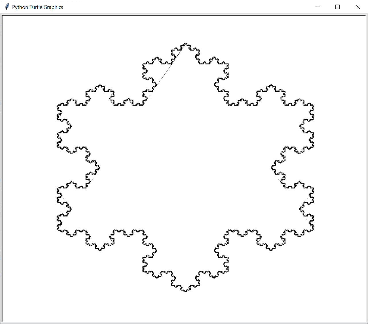
Koch Snowflake Fractal
First introduced in 1902 by Swedish mathematician Helge von Koch, the Koch curve is one of the earliest fractals to be described mathematically. Its construction is simple: take a line of length b and divide it into three equal parts, each of length b / 3. Replace the middle section with a “bump” whose sides are also of length b / 3. This bump causes the Koch curve to be longer than the original line, since there are now four line segments of length b / 3. (We’ll exclude the original middle part of the line segment.) This bump-creation can be repeated on the new four line segments. The Koch Snowflake is three of these Koch curves connected together.
The output of this program looks like this:
Merge Sort
Computer scientist John von Neumann developed merge sort in 1945 and it is an efficient, general-purpose sorting algorithm particularly used to sort linked list data structures. It uses a divide-merge approach: each recursive call to mergeSort() divides the unsorted list into halves until they’ve been whittled down into lists with lengths of zero or one. Then, as the recursive calls return, these smaller lists are merged together into sorted order. When the last recursive call has returned, the entire list will have been sorted.
For example, the divide step takes a list, such as [0, 7, 6, 3, 1, 2, 5, 4], and splits it into two lists, like [0, 7, 6, 3] and [1, 2, 5, 4], to pass to two recursive function calls. At the base case, the lists have been divided into lists of zero or one item. After the recursive calls return, the code merges the two lists into a larger list. If the two lists are in sorted order (and lists of zero or one item are sorted by their nature), merging will also produce a sorted list. The end result is that the original mergeSort() call returns the full list in sorted order.
The output of this program looks like this:
Permutations
A permutation of a set is a specific ordering of all elements in the set. For example, there are six permutations for the set {A, B, C}: ABC, ACB, BAC, BCA, CAB, and CBA. We call these permutations without repetition or permutations without replacement, because each element doesn’t appear in the permutation more than once.
Imagine you must arrange the seating chart for a wedding reception with delicate social requirements. Some of the guests hate each other and while others demand to sit near an influential guest. The seats at the table form one long row, rather than a circle. It’d be helpful for your planning to see every possible ordering of guests, that is, every permutation without repetition of the set of guests. There is no repetition because each guest will only appear in the seating chart once. Let’s use a simple example of Alice, Bob, and Carol, or {A, B, C}.
The output of this program looks like this:
Quicksort
Quicksort uses a divide-and-conquer technique called partitioning. Think of partitioning this way: imagine you have a large pile of unalphabetized books. Grabbing one book and placing it in the right spot on the shelf means you’ll spend a lot of time rearranging the bookshelf as it gets full. It would help if you first turned the pile of books into two piles: an A to M pile and an N to Z pile. (In this example, M would be our pivot.)
You haven’t sorted the pile, but you have partitioned it. And partitioning is easy: the book doesn’t have to go into the correct place in one of the two piles, it just has to go into the correct pile. Then you can further partition these two piles into four piles: A to G, H to M, N to T, and U to Z. This is shown in Figure 5-x. If you keep partitioning, you end up with piles that contain one book each (the base case), and the piles are now in sorted order. This repeated partitioning is how quicksort works.
In our implementation, each call to quicksort() is given an array of items to sort. It is also given left and right arguments specifying the range of indexes in that array to sort, similar to binarySearch()’s left and right arguments. The algorithm selects a pivot value to compare with the other values in the range, then places the values to either the left side of the range (if they’re less than the pivot value) or the right side (if they’re greater than the pivot value). This is the partition step. Next, the quicksort() function is recursively called on these two, smaller ranges until a range has been reduced to zero. The list becomes more and more sorted as the recursive calls are made, until finally the entire list is in correct order.
The output of this program looks like this:
Shortest Possible Recursive Function
For a demonstration, this is the shortest possible recursive function. It is merely a function that calls itself. It will result in a stack overflow error.
The output of this program looks like this:
Sierpinski Carpet
The sierpinski carpet is a square with an empty center and fractal sierpinski carpets in the eight perimeter areas of the square.
The output of this program looks like this:

Sierpinski Triangle
Download sierpinskiTriangle.py
The sierpinski triangle is an equilateral triangle that contains three sierpinski triangles. It looks like the triforce from Zelda video games.
The output of this program looks like this:

Towers of Hanoi
Download towerOfHanoiSolver.py
The Tower of Hanoi is a puzzle involving a tower of stacked disks. The puzzle begins with the largest disk on the bottom and the disk sizes decrease going up. The disks have a hole in their center so they can be stacked on top of each other through a pole. To solve the puzzle, the player must move the stack of disks from one pole to another while following three rules:
- The player can move only one disk at a time.
- The player can only move disks to and from the top of a tower.
- The player can never place a larger disk on top of a smaller disk.
The output of this program looks like this:
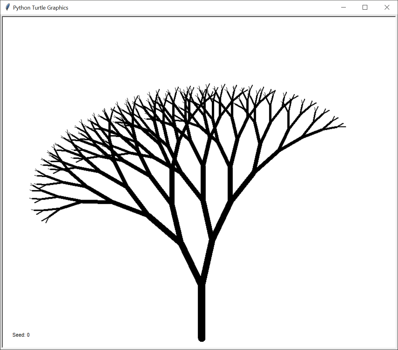
Tree Fractal
Trees can be algorithmically generated as a fractal. These trees are generated by having each branch produce two more similar but smaller branches.
The output of this program looks like this:
Learn More About Recursion
To learn how these programs work and learn more about recursion in general, you can check out my book, The Recursive Book of Recursion. You can get an ebook copy for free when you buy a print book from the publisher, No Starch Press.
