Check out other books by Al Sweigart, free online or available for purchase:
...and other books as well! Or register for the online video course. You can also donate to support the author directly.


Certainly, the most fun application of recursion is drawing fractals. Fractals are shapes that repeat themselves, sometimes chaotically, at different scales. The term was coined by the founder of fractal geometry, Benoit B. Mandelbrot, in 1975 and is derived from the Latin frāctus, meaning broken or fractured, like shattered glass. Fractals include many natural and artificial shapes. In nature, you might see them in the shapes of trees, fern leaves, mountain ranges, lightning bolts, coastlines, river networks, and snowflakes. Mathematicians, programmers, and artists can create elaborate geometric shapes based on a few recursive rules.
Recursion can produce elaborate fractal art using surprisingly few lines of code. This chapter covers Python’s built-in turtle module for generating several common fractals with code. To create turtle graphics with JavaScript, you can use Greg Reimer’s jtg library. For simplicity, this chapter presents only the Python fractal drawing programs and not the JavaScript equivalents. However, the jtg JavaScript library is covered in this chapter.
Turtle graphics were a feature of the Logo programming language designed to help kids learn coding concepts. The feature has since been reproduced in many languages and platforms. Its central idea is an object called a turtle.
The turtle acts as a programmable pen that draws lines in a 2D window. Imagine an actual turtle holding a pen on the ground, drawing a line behind it as it moves around. The turtle can adjust the size and color of its pen, or “raise the pen” so that it does not draw as it moves. Turtle programs can produce intricate geometric drawings such as Figure 9-1.
When you put these instructions inside loops and functions, even small programs can create impressive geometric drawings. Consider the following spiral.py program:
Python
import turtle
turtle.tracer(1, 0) # Makes the turtle draw faster.
for i in range(360):
    turtle.forward(i)
    turtle.left(59)
turtle.exitonclick() # Pause until user clicks in the window.
When you run this program, the turtle window opens. The turtle (represented by a triangle) will trace the spiral pattern in Figure 9-1. While not a fractal, it is a beautiful drawing.
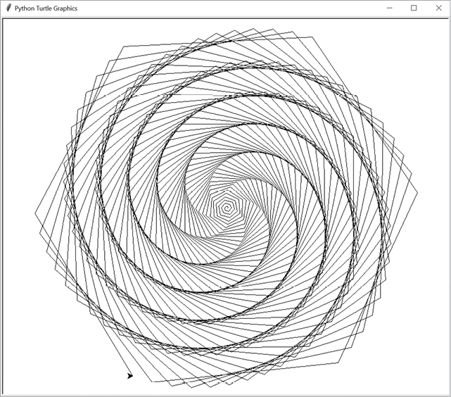
Figure 9-1: The spiral drawn by the program using Python’s turtle module
The window in a turtle graphics system uses Cartesian x- and y-coordinates. The number for the horizontal x-coordinate increases going right and decreases going left, while the number for the vertical y-coordinate increases going up and decreases going down. These two coordinates together can provide a unique address for any point in the window. By default, the origin (the x, y coordinate point at 0, 0) is in the center of the window.
The turtle also has a heading, or direction, that is a number from 0 to 359 (a circle is split into 360 degrees). In Python’s turtle module, a heading of 0 faces east (toward the right edge of the screen) and increases counterclockwise; a heading of 90 faces north, a heading of 180 faces west, and a heading of 270 faces south. In the JavaScript jtg library, this orientation is rotated so that 0 degrees faces north and increases clockwise. Figure 9-2 demonstrates the headings for the Python turtle module and the JavaScript jtg library.
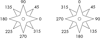
Figure 9-2: The headings in Python’s turtle module (left) and the JavaScript jtg library (right)
In the JavaScript jtg library at https://inventwithpython.com/jtg, enter the following code into the text field at the bottom of the page:
JavaScript
for (let i = 0; i < 360; i++) { t.fd(i); t.lt(59) }This draws the same spiral shown in Figure 9-1 on the main area of the web page.
The most commonly used functions in turtle graphics cause the turtle to change heading and move forward or backward. The turtle.left() and turtle.right() functions rotate the turtle a certain number of degrees starting from its current heading, while the turtle.forward() and turtle.backward() functions move the turtle based on its current position.
Table 9-1 lists some of the turtle’s functions. The first function (beginning with turtle.) is for Python, and the second (beginning with t.) is for JavaScript. The full Python documentation is available at https://docs.python.org/3/library/turtle.html. In the JavaScript jtg software, you can press F1 to display the help screen.
Table 9-1: Turtle Functions in Python’s turtle Module and JavaScript’s jtg Library
| Python | JavaScript | Description |
goto(x, y) |
xy(x, y) |
Moves the turtle to the x, y coordinates. |
setheading(deg) |
heading(deg) |
Sets the turtle’s heading. In Python, 0 degrees is east (right). In JavaScript, 0 degrees is north (up). |
forward(steps) |
fd(steps) |
Moves the turtle a number of steps forward in the heading it is facing. |
backward(steps) |
bk(steps) |
Moves the turtle a number of steps in the heading opposite from the one it is facing. |
left(deg) |
lt(deg) |
Turns the turtle’s heading to the left. |
right(deg) |
rt(deg) |
Turns the turtle’s heading to the right. |
penup() |
pu() |
“Raises the pen” so that the turtle stops drawing as it moves. |
pendown() |
pd() |
“Lowers the pen” so that the turtle starts drawing as it moves. |
pensize(size) |
thickness(size) |
Changes the thickness of the lines the turtle draws. The default is 1. |
pencolor(color) |
color(color) |
Changes the color of the lines the turtle draws. This can be a string of a common color such as red or white. The default is black. |
xcor() |
get.x() |
Returns the turtle’s current x position. |
ycor() |
get.y() |
Returns the turtle’s current y position. |
heading() |
get.heading() |
Returns the turtle’s current heading as a floating-point number from 0 to 359. In Python, 0 degrees is east (right). In JavaScript, 0 degrees is north (up). |
reset() |
reset() |
Clears any drawn lines, and moves the turtle back to the original position and heading. |
clear() |
clean() |
Clears any drawn lines but doesn’t move the turtle. |
The functions listed in Table 9-2 are available only in the Python turtle module.
Table 9-2: Python-Only Turtle Functions
| Python | Description |
begin_fill() |
Begins drawing a filled-in shape. The lines drawn after this call will specify the perimeter of the filled-in shape. |
end_fill() |
Draws the filled-in shape that was started with the call to turtle.begin_fill(). |
fillcolor(color) |
Sets the color used for filled-in shapes. |
hideturtle() |
Hides the triangle that represents the turtle. |
showturtle() |
Shows the triangle that represents the turtle. |
tracer(drawingUpdates, delay) |
Adjusts the speed of drawing. Pass 0 for delay for a delay of 0 milliseconds after each line the turtle draws. The larger the number passed for drawingUpdates, the faster the turtle draws by increasing the number of drawings before the module updates the screen. |
update() |
Draws any buffered lines (explained later in this section) to the screen. Call this after the turtle has completed drawing. |
setworldcoordinates(llx, lly, urx, ury) |
Readjusts which part of the coordinate plane the window shows. The first two arguments are the x, y coordinates for the lower-left corner of the window. The latter two arguments are the x, y coordinates for the upper-right corner of the window. |
exitonclick() |
Pauses the program and closes the window when the user clicks anywhere. Without this at the end of your program, the turtle graphics window may close as soon as the program ends. |
In Python’s turtle module, lines are displayed on the screen immediately. However, this can slow programs that draw thousands of lines. It’s faster to buffer—that is, hold off displaying several lines and then display them all at once.
By calling turtle.tracer(1000, 0), you can instruct the turtle module to hold off displaying lines until 1,000 lines have been created by your program. After your program has finished calling line-drawing functions, make a final call to turtle.update() to display any remaining buffered lines to the screen. If your program is still taking too long to draw an image, pass a larger integer such as 2000 or 10000 as the first argument to turtle.tracer().
The easiest fractal to draw on paper is the Sierpiński triangle, introduced in Chapter 1. This fractal was described by Polish mathematician Wacław Sierpiński in 1915 (predating even the term fractal). However, the pattern is at least hundreds of years older.
To create a Sierpiński triangle, start by drawing an equilateral triangle—a triangle with equal-length sides, like the one on the left in Figure 9-3. Then draw an upside-down equilateral triangle inside the first triangle, as on the right in Figure 9-3. You’ll form a shape that, if you’re familiar with the Legend of Zelda video games, looks like the Triforce.

Figure 9-3: An equilateral triangle (left) with an upside-down triangle added to form a Sierpiński triangle, with additional triangles recursively added
An interesting thing happens when you draw the inner, upside-down triangle. You form three new, right-side-up equilateral triangles. Inside each of these three triangles, you can draw another upside-down triangle, which will create nine triangles. This recursion can continue forever mathematically, though in reality your pen won’t be able to keep drawing tinier triangles.
This property, describing a full object that is similar to a part of itself, is called self-similarity. Recursive functions can produce these objects, since they “call” themselves again and again. Practically, this code must hit a base case eventually, but mathematically, these shapes have infinite resolution: you could theoretically zoom in on the shape forever.
Let’s write a recursive program to create the Sierpiński triangle. The recursive drawTriangle() function will draw an equilateral triangle, and then recursively call this function three times to draw the inner equilateral triangles, as in Figure 9-4. The midpoint() function finds the point equidistant from two points passed to the function. This will be important as the inner triangles use these equidistant points for their vertices.

Figure 9-4: The three inner triangles, with midpoints shown with large dots
Note that this program calls turtle.setworldcoordinates(0, 0, 700, 700), which makes the 0, 0 origin at the lower-left corner of the window. The upper-right corner has the x, y coordinates 700, 700. The source code for sierpinskiTriangle.py is as follows:
import turtle
turtle.tracer(100, 0) # Increase the first argument to speed up the drawing.
turtle.setworldcoordinates(0, 0, 700, 700)
turtle.hideturtle()

MIN_SIZE = 4 # Try changing this to decrease/increase the amount of recursion.

def midpoint(startx, starty, endx, endy):
    # Return the x, y coordinate in the middle of the four given parameters.
    xDiff = abs(startx - endx)
    yDiff = abs(starty - endy)
    return (min(startx, endx) + (xDiff / 2.0), min(starty, endy) + (yDiff / 2.0))

def isTooSmall(ax, ay, bx, by, cx, cy):
    # Determine if the triangle is too small to draw.
    width = max(ax, bx, cx) - min(ax, bx, cx)
    height = max(ay, by, cy) - min(ay, by, cy)
    return width < MIN_SIZE or height < MIN_SIZE

def drawTriangle(ax, ay, bx, by, cx, cy):
    if isTooSmall(ax, ay, bx, by, cx, cy):
        # BASE CASE
        return
    else:
        # RECURSIVE CASE
        # Draw the triangle.
        turtle.penup()
        turtle.goto(ax, ay)
        turtle.pendown()
        turtle.goto(bx, by)
        turtle.goto(cx, cy)
        turtle.goto(ax, ay)
        turtle.penup()

        # Calculate midpoints between points A, B, and C.
        mid_ab = midpoint(ax, ay, bx, by)
        mid_bc = midpoint(bx, by, cx, cy)
        mid_ca = midpoint(cx, cy, ax, ay)

        # Draw the three inner triangles.
        drawTriangle(ax, ay, mid_ab[0], mid_ab[1], mid_ca[0], mid_ca[1])
        drawTriangle(mid_ab[0], mid_ab[1], bx, by, mid_bc[0], mid_bc[1])
        drawTriangle(mid_ca[0], mid_ca[1], mid_bc[0], mid_bc[1], cx, cy)
        return

# Draw an equilateral Sierpinski triangle.
drawTriangle(50, 50, 350, 650, 650, 50)

# Draw a skewed Sierpinski triangle.
#drawTriangle(30, 250, 680, 600, 500, 80)

turtle.exitonclick()
When you run this code, the output looks like Figure 9-5.
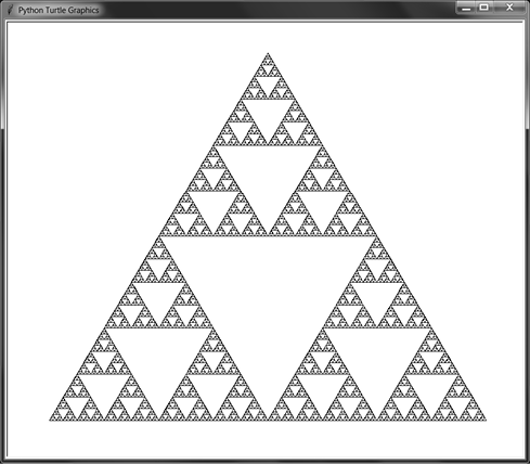
Figure 9-5: A standard Sierpiński triangle
Sierpiński triangles don’t have to be drawn with equilateral triangles. As long as you use the midpoints of the outer triangle to draw the inner triangles, you can use any kind of triangle. Comment out the first drawTriangle() call and uncomment the second one (under the # Draw a skewed Sierpinski triangle. comment) and run the program again. The output will look like Figure 9-6.
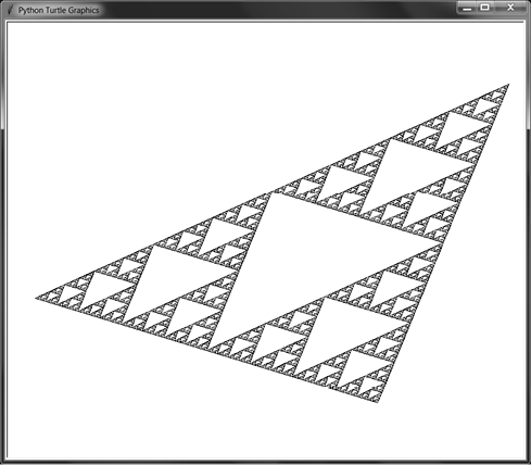
Figure 9-6: A skewed Sierpiński triangle
The drawTriangle() function takes six arguments corresponding to the x, y coordinates of the triangle’s three points. Try experimenting with different values to adjust the shape of the Sierpiński triangle. You can also change the MIN_SIZE constant to a larger value to make the program reach the base case sooner and reduce the number of triangles drawn.
A fractal shape similar to the Sierpiński triangle can be drawn using rectangles instead. This pattern is known as the Sierpiński carpet. Imagine splitting a black rectangle into a 3 × 3 grid, then “cutting out” the center rectangle. Repeat this pattern in the surrounding eight rectangles of the grid. When this is done recursively, you end up with a pattern like Figure 9-7.
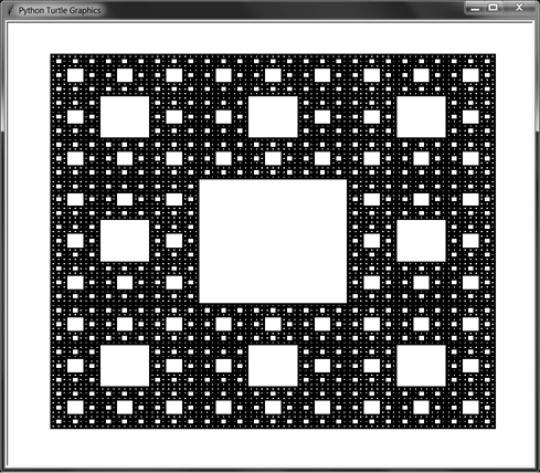
Figure 9-7: The Sierpiński carpet
The Python program that draws the carpet uses the turtle.begin_fill() and turtle.end_fill() functions to create solid, filled-in shapes. The lines that the turtle draws between these calls are used to draw the shape, as in Figure 9-8.

Figure 9-8: Calling turtle.begin_fill(), drawing a path, and calling turtle.end_fill() creates a filled-in shape.
The base case is reached when the rectangles of the 3 × 3 become smaller than six steps on a side. You can change the MIN_SIZE constant to a larger value to make the program reach the base case sooner. The source code for sierpinskiCarpet.py is as follows:
import turtle
turtle.tracer(10, 0) # Increase the first argument to speed up the drawing.
turtle.setworldcoordinates(0, 0, 700, 700)
turtle.hideturtle()

MIN_SIZE = 6 # Try changing this to decrease/increase the amount of recursion.
DRAW_SOLID = True

def isTooSmall(width, height):
    # Determine if the rectangle is too small to draw.
    return width < MIN_SIZE or height < MIN_SIZE

def drawCarpet(x, y, width, height):
    # The x and y are the lower-left corner of the carpet.

    # Move the pen into position.
    turtle.penup()
    turtle.goto(x, y)

    # Draw the outer rectangle.
    turtle.pendown()
    if DRAW_SOLID:
        turtle.fillcolor('black')
        turtle.begin_fill()
    turtle.goto(x, y + height)
    turtle.goto(x + width, y + height)
    turtle.goto(x + width, y)
    turtle.goto(x, y)
    if DRAW_SOLID:
        turtle.end_fill()
    turtle.penup()

    # Draw the inner rectangles.
    drawInnerRectangle(x, y, width, height)

def drawInnerRectangle(x, y, width, height):
    if isTooSmall(width, height):
        # BASE CASE
        return
    else:
        # RECURSIVE CASE

        oneThirdWidth = width / 3
        oneThirdHeight = height / 3
        twoThirdsWidth = 2 * (width / 3)
        twoThirdsHeight = 2 * (height / 3)

        # Move into position.
        turtle.penup()
        turtle.goto(x + oneThirdWidth, y + oneThirdHeight)

        # Draw the inner rectangle.
        if DRAW_SOLID:
            turtle.fillcolor('white')
            turtle.begin_fill()
        turtle.pendown()
        turtle.goto(x + oneThirdWidth, y + twoThirdsHeight)
        turtle.goto(x + twoThirdsWidth, y + twoThirdsHeight)
        turtle.goto(x + twoThirdsWidth, y + oneThirdHeight)
        turtle.goto(x + oneThirdWidth, y + oneThirdHeight)
        turtle.penup()
        if DRAW_SOLID:
            turtle.end_fill()

        # Draw the inner rectangles across the top.
        drawInnerRectangle(x, y + twoThirdsHeight, oneThirdWidth, oneThirdHeight)
        drawInnerRectangle(x + oneThirdWidth, y + twoThirdsHeight, oneThirdWidth, oneThirdHeight)
        drawInnerRectangle(x + twoThirdsWidth, y + twoThirdsHeight, oneThirdWidth, oneThirdHeight)

        # Draw the inner rectangles across the middle.
        drawInnerRectangle(x, y + oneThirdHeight, oneThirdWidth,
        oneThirdHeight)
        drawInnerRectangle(x + twoThirdsWidth, y + oneThirdHeight, oneThirdWidth,
        oneThirdHeight)

        # Draw the inner rectangles across the bottom.
        drawInnerRectangle(x, y, oneThirdWidth, oneThirdHeight)
        drawInnerRectangle(x + oneThirdWidth, y, oneThirdWidth, oneThirdHeight)
        drawInnerRectangle(x + twoThirdsWidth, y, oneThirdWidth,
        oneThirdHeight)

drawCarpet(50, 50, 600, 600)
turtle.exitonclick()
You can also set the DRAW_SOLID constant to False and run the program. This will skip the calls to turtle.begin_fill() and turtle.end_fill() so that only the outlines of the rectangles are drawn, as in Figure 9-9.
Try passing different arguments to drawCarpet(). The first two arguments are the x, y coordinates of the lower-left corner of the carpet, while the latter two arguments are the width and height. You can also change the MIN_SIZE constant to a larger value to make the program reach the base case sooner and reduce the number of rectangles drawn.
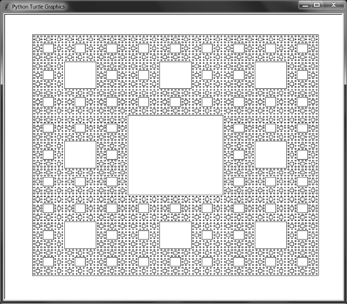
Figure 9-9: The Sierpiński carpet, with only the outlines of the rectangles drawn
Another 3D Sierpiński carpet uses cubes instead of squares. In this form, it is called a Sierpiński cube, or Menger sponge. It was first described by mathematician Karl Menger in 1926. Figure 9-10 shows a Menger sponge created in the video game Minecraft.
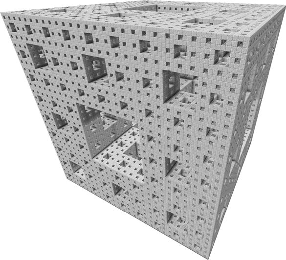
Figure 9-10: A 3D Menger sponge fractal
While the artificial fractals such as the Sierpiński triangle and carpet are perfectly self-similar, fractals can include shapes that do not have perfect self-similarity. Fractal geometry, as envisioned by mathematician Benoit B. Mandelbrot (whose middle initial recursively stands for Benoit B. Mandelbrot) included natural shapes such as mountains, coastlines, plants, blood vessels, and the clustering of galaxies as fractals. Upon close examination, these shapes continued to consist of “rougher” shapes not easily contained by the smooth curves and straight lines of simplified geometry.
As an example, we can use recursion to reproduce fractal trees, whether perfectly or imperfectly self-similar. Generating trees requires creating a branch with two child branches that issue from their parent at set angles and decrease at set lengths. The Y shape that they produce is recursively repeated to create a convincing drawing of a tree, as in Figures 9-11 and 9-12.
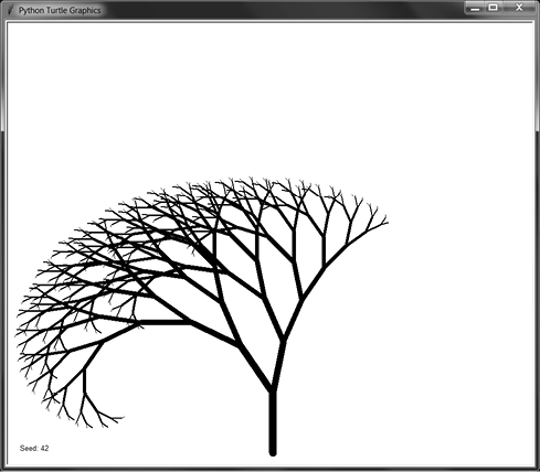
Figure 9-11: A perfectly self-similar fractal tree generated with the left and right branches using consistent angles and lengths
Movies and video games can use such recursive algorithms in procedural generation, the automatic (rather than manual) creation of 3D models such as trees, ferns, flowers, and other plants. Using algorithms, computers can quickly create entire forests consisting of millions of unique trees, saving an army of human 3D artists the painstaking effort.
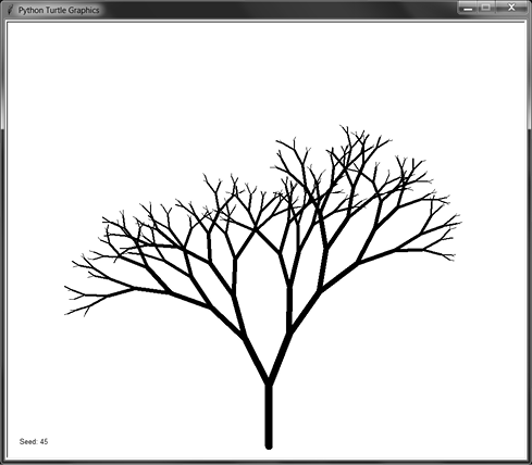
Figure 9-12: A more realistic tree created using random changes to branch angle and lengths
Our fractal tree program displays a new, randomly generated tree every two seconds. The source code for fractalTree.py is as follows:
Python
import random
import time
import turtle
turtle.tracer(1000, 0) # Increase the first argument to speed up the drawing.
turtle.setworldcoordinates(0, 0, 700, 700)
turtle.hideturtle()

def drawBranch(startPosition, direction, branchLength):
    if branchLength < 5:
        # BASE CASE
        return

    # Go to the starting point & direction.
    turtle.penup()
    turtle.goto(startPosition)
    turtle.setheading(direction)

    # Draw the branch (thickness is 1/7 the length).
    turtle.pendown()
    turtle.pensize(max(branchLength / 7.0, 1))
    turtle.forward(branchLength)

    # Record the position of the branch's end.
    endPosition = turtle.position()
    leftDirection = direction + LEFT_ANGLE
    leftBranchLength = branchLength - LEFT_DECREASE
    rightDirection = direction - RIGHT_ANGLE
    rightBranchLength = branchLength - RIGHT_DECREASE

    # RECURSIVE CASE
    drawBranch(endPosition, leftDirection, leftBranchLength)
    drawBranch(endPosition, rightDirection, rightBranchLength)

seed = 0
while True:
    # Get pseudorandom numbers for the branch properties.
    random.seed(seed)
    LEFT_ANGLE     = random.randint(10,  30)
    LEFT_DECREASE  = random.randint( 8,  15)
    RIGHT_ANGLE    = random.randint(10,  30)
    RIGHT_DECREASE = random.randint( 8,  15)
    START_LENGTH   = random.randint(80, 120)

    # Write out the seed number.
    turtle.clear()
    turtle.penup()
    turtle.goto(10, 10)
    turtle.write('Seed: %s' % (seed))

    # Draw the tree.
    drawBranch((350, 10), 90, START_LENGTH)
    turtle.update()
    time.sleep(2)

    seed = seed + 1
This program produces perfectly self-similar trees, as the LEFT_ANGLE, LEFT_DECREASE, RIGHT_ANGLE, and RIGHT_DECREASE variables are initially randomly chosen but stay constant for all the recursive calls. The random.seed() function sets a seed value for Python’s random functions. The random number seed value causes the program to produce random-seeming numbers, but it uses the same sequence of random numbers for each branch of the tree. In other words, the same seed value reproduces the same tree each time you run the program. (I never apologize for my puns.)
To see this in action, enter the following into the Python interactive shell:
Python
>>> import random
>>> random.seed(42)
>>> [random.randint(0, 9) for i in range(20)]
 [1, 0, 4, 3, 3, 2, 1, 8, 1, 9, 6, 0, 0, 1, 3, 3, 8, 9, 0, 8]
>>> [random.randint(0, 9) for i in range(20)]
 [3, 8, 6, 3, 7, 9, 4, 0, 2, 6, 5, 4, 2, 3, 5, 1, 1, 6, 1, 5]
>>> random.seed(42)
>>> [random.randint(0, 9) for i in range(20)]
 [1, 0, 4, 3, 3, 2, 1, 8, 1, 9, 6, 0, 0, 1, 3, 3, 8, 9, 0, 8]
In this example, we set the random seed to 42. When we generate 20 random integers, we get 1, 0, 4, 3, and so on. We can generate another 20 integers and continue to receive random integers. However, if we reset the seed to 42 and generate 20 random integers again, they’ll be the same “random” integers as before.
If you’d like to create a more natural, less self-similar tree, replace the lines after the # Record the position of the branch's end. comment with the following lines. This generates new random angles and branch lengths for every recursive call, which is closer to the way trees grow in nature:
Python
    # Record the position of the branch's end.
    endPosition = turtle.position()
    leftDirection = direction + random.randint(10, 30)
    leftBranchLength = branchLength - random.randint(8, 15)
    rightDirection = direction - random.randint(10, 30)
    rightBranchLength = branchLength - random.randint(8, 15)
You can experiment with different ranges for the random.randint() call, or try adding more recursive calls instead of just the two for the two branches.
Before I tell you about the Koch curve and snowflake, consider this question: how long is the coast of Great Britain? Look at Figure 9-13. The map on the left has a rough measure, which puts the coast at about 2,000 miles. But the map on the right has a more precise measure, which includes more nooks and crannies of the coast and comes to about 2,800 miles.
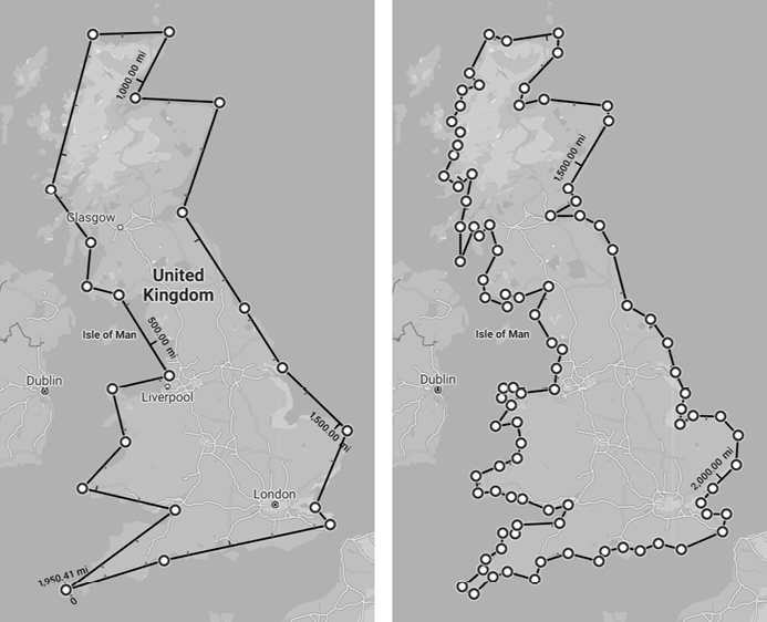
Figure 9-13: The island of Great Britain, with a rough measure (left) and more precise measure (right). Measuring the coast more precisely adds 800 miles to its length.
Mandelbrot’s key insight about fractals such as the coastline of Britain is that you can continue to look closer and closer, and there will continue to be “roughness” at every scale. So, as your measurement gets finer and finer, the length of the coastline will get longer and longer. The “coast” will follow the Thames upriver, deep into the landmass along one bank and back out to the English Channel on the other bank. Thus, the answer to our question of Great Britain’s coastline’s length is, “It depends.”
The Koch curve fractal has a similar property pertaining to the length of its coastline, or rather, perimeter. First introduced in 1902 by Swedish mathematician Helge von Koch, the Koch curve is one of the earliest fractals to be described mathematically. To construct it, take a line of length b and divide it into three equal parts, each of length b / 3. Replace the middle section with a “bump” whose sides are also of length b / 3. This bump causes the Koch curve to be longer than the original line, since we now have four line segments of length b / 3. (We’ll exclude the original middle part of the line segment.) This bump creation can be repeated on the new four line segments. Figure 9-14 shows this construction.
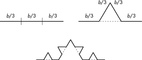
Figure 9-14: After splitting the line segment into three equal parts (left), add a bump to the middle part (right). We now have four segments of length b / 3, to which bumps can be added again (bottom).
To create the Koch snowflake, we start with an equilateral triangle and construct three Koch curves from its three sides, as in Figure 9-15.
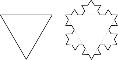
Figure 9-15: Creating three Koch curves on the three sides of an equilateral triangle to form a Koch snowflake
Each time you create a new bump, you are increasing the curve’s length from three b / 3 lengths to four b / 3 lengths, or 4b / 3. If you continue to do this with the three sides of an equilateral triangle, you’ll create the Koch snowflake, as in Figure 9-16. (The small dotted patterns are artifacts, because slight rounding errors cause the turtle module to be unable to completely erase the middle b / 3 segment.) You can continue to create new bumps forever, though our program stops when they get smaller than a few pixels.
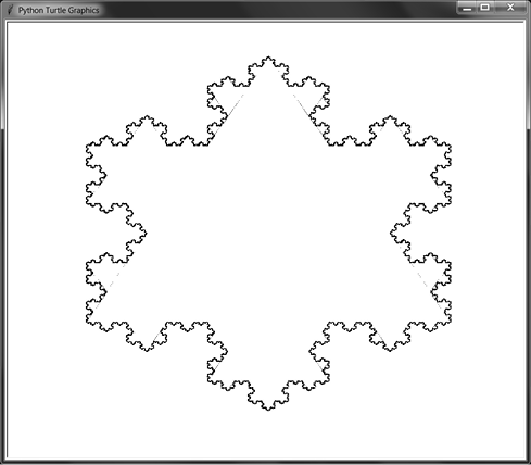
Figure 9-16: A Koch snowflake. Some of the interior lines remain because of small rounding errors.
The source code for kochSnowflake.py is as follows:
Python
import turtle
turtle.tracer(10, 0) # Increase the first argument to speed up the drawing.
turtle.setworldcoordinates(0, 0, 700, 700)
turtle.hideturtle()
turtle.pensize(2)

def drawKochCurve(startPosition, heading, length):
    if length < 1:
        # BASE CASE
        return
    else:
        # RECURSIVE CASE
        # Move to the start position.
        recursiveArgs = []
        turtle.penup()
        turtle.goto(startPosition)
        turtle.setheading(heading)
        recursiveArgs.append({'position':turtle.position(),
                              'heading':turtle.heading()})

        # Erase the middle third.
        turtle.forward(length / 3)
        turtle.pencolor('white')
        turtle.pendown()
        turtle.forward(length / 3)

        # Draw the bump.
        turtle.backward(length / 3)
        turtle.left(60)
        recursiveArgs.append({'position':turtle.position(),
                              'heading':turtle.heading()})
        turtle.pencolor('black')
        turtle.forward(length / 3)
        turtle.right(120)
        recursiveArgs.append({'position':turtle.position(),
                              'heading':turtle.heading()})
        turtle.forward(length / 3)
        turtle.left(60)
        recursiveArgs.append({'position':turtle.position(),
                              'heading':turtle.heading()})

        for i in range(4):
            drawKochCurve(recursiveArgs[i]['position'],
                     recursiveArgs[i]['heading'],
                     length / 3)
        return

def drawKochSnowflake(startPosition, heading, length):
    # A Koch snowflake is three Koch curves in a triangle.

    # Move to the starting position.
    turtle.penup()
    turtle.goto(startPosition)
    turtle.setheading(heading)

    for i in range(3):
        # Record the starting position and heading.
        curveStartingPosition = turtle.position()
        curveStartingHeading = turtle.heading()
        drawKochCurve(curveStartingPosition,
                      curveStartingHeading, length)

        # Move back to the start position for this side.
        turtle.penup()
        turtle.goto(curveStartingPosition)
        turtle.setheading(curveStartingHeading)

        # Move to the start position of the next side.
        turtle.forward(length)
        turtle.right(120)

drawKochSnowflake((100, 500), 0, 500)
turtle.exitonclick()
The Koch snowflake is also sometimes called the Koch island. Its coastline would be literally infinitely long. While the Koch snowflake fits into the finite area of a page of this book, the length of its perimeter is infinite, proving that, while it seems counterintuitive, the finite can contain the infinite!
A space-filling curve is a 1D line that curves around until it completely fills a 2D space without crossing over itself. German mathematician David Hilbert described his space-filling Hilbert curve in 1891. If you split a 2D area into a grid, the single, 1D line of the Hilbert curve can run through every cell in the grid.
Figure 9-17 contains the first three recursions of the Hilbert curve. The next recursion contains four copies of the previous recursion, and the dashed line shows how the four copies connect to one another.

Figure 9-17: The first three recursions of the Hilbert space-filling curve
As the cells become infinitesimal points, the 1D curve can fill the entire 2D space the same way a 2D square does. Counterintuitively, this creates a 2D shape from a strictly 1D line!
The source code for hilbertCurve.py is as follows:
Python
import turtle
turtle.tracer(10, 0) # Increase the first argument to speed up the drawing.
turtle.setworldcoordinates(0, 0, 700, 700)
turtle.hideturtle()

LINE_LENGTH  = 5 # Try changing the line length by a little.
ANGLE = 90 # Try changing the turning angle by a few degrees.
LEVELS = 6 # Try changing the recursive level by a little.
DRAW_SOLID = False
#turtle.setheading(20) # Uncomment this line to draw the curve at an angle.

def hilbertCurveQuadrant(level, angle):
    if level == 0:
        # BASE CASE
        return
    else:
        # RECURSIVE CASE
        turtle.right(angle)
        hilbertCurveQuadrant(level - 1, -angle)
        turtle.forward(LINE_LENGTH)
        turtle.left(angle)
        hilbertCurveQuadrant(level - 1, angle)
        turtle.forward(LINE_LENGTH)
        hilbertCurveQuadrant(level - 1, angle)
        turtle.left(angle)
        turtle.forward(LINE_LENGTH)
        hilbertCurveQuadrant(level - 1, -angle)
        turtle.right(angle)
        return

def hilbertCurve(startingPosition):
    # Move to starting position.
    turtle.penup()
    turtle.goto(startingPosition)
    turtle.pendown()
    if DRAW_SOLID:
        turtle.begin_fill()

    hilbertCurveQuadrant(LEVELS, ANGLE) # Draw lower-left quadrant.
    turtle.forward(LINE_LENGTH)

    hilbertCurveQuadrant(LEVELS, ANGLE) # Draw lower-right quadrant.
    turtle.left(ANGLE)
    turtle.forward(LINE_LENGTH)
    turtle.left(ANGLE)

    hilbertCurveQuadrant(LEVELS, ANGLE) # Draw upper-right quadrant.
    turtle.forward(LINE_LENGTH)

    hilbertCurveQuadrant(LEVELS, ANGLE) # Draw upper-left quadrant.

    turtle.left(ANGLE)
    turtle.forward(LINE_LENGTH)
    turtle.left(ANGLE)
    if DRAW_SOLID:
        turtle.end_fill()

hilbertCurve((30, 350))
turtle.exitonclick()
Try experimenting with this code by decreasing LINE_LENGTH to shorten the line segments while increasing LEVELS to add more levels of recursion. Because this program uses only relative movements for the turtle, you can uncomment the turtle.setheading(20) line to draw the Hilbert curve at a 20-degree angle. Figure 9-18 shows the drawing produced with LINE_LENGTH of 10 and LEVELS of 5.
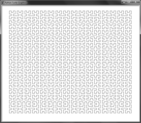
Figure 9-18: Five levels of the Hilbert curve, with line length 10
The Hilbert curve makes 90-degree (right-angle) turns. But try adjusting the ANGLE variable by a few degrees to 89 or 86, and run the program to view the changes. You can also set the DRAW_SOLID variable to True to produce a filled-in Hilbert curve, as in Figure 9-19.
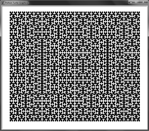
Figure 9-19: Six levels of the Hilbert curve, filled in, with line length 5
The incredibly wide field of fractals combines all the most interesting parts of programming and art, making this chapter the most fun to write. Mathematicians and computer scientists talk about the beauty and elegance that the advanced topics of their fields produce, but recursive fractals are able to turn this conceptual beauty into visual beauty that anyone can appreciate.
This chapter covered several fractals and the programs that draw them: the Sierpiński triangle, the Sierpiński carpet, procedurally generated fractal trees, the Koch curve and snowflake, and the Hilbert curve. All of these were drawn with Python’s turtle module and functions that recursively call themselves.
To learn more about drawing with Python’s turtle module, I’ve written a simple tutorial at https://github.com/asweigart/simple-turtle-tutorial-for-python. I also have a personal collection of turtle programs at https://github.com/asweigart/art-of-turtle-programming.
The question of Great Britain’s coastline’s length came from the title of a 1967 paper by Mandelbrot. The idea is summarized nicely on Wikipedia at https://en.wikipedia.org/wiki/Coastline_paradox. Khan Academy has more on the geometry of the Koch snowflake at https://www.khanacademy.org/math/geometry-home/geometry-volume-surface-area/koch-snowflake/v/koch-snowflake-fractal.
The 3Blue1Brown YouTube channel has excellent animations of fractals, particularly the “Fractals Are Typically Not Self-Similar” video at https://youtu.be/gB9n2gHsHN4 and the “Fractal Charm: Space-Filling Curves” video at https://youtu.be/RU0wScIj36o.
Other space-filling curves require recursion to draw, such as the Peano curve, Gosper curve, and dragon curve, and they’re worth researching on the web.
Test your comprehension by answering the following questions:
For practice, write a program for each of the following tasks:
turtle.begin_fill() and turtle.end_fill() functions to draw the first large, black square. Then split this square into nine equal sections, and draw white squares in the top, left, right, and bottom squares. Repeat this process for the four corner squares and the center square.
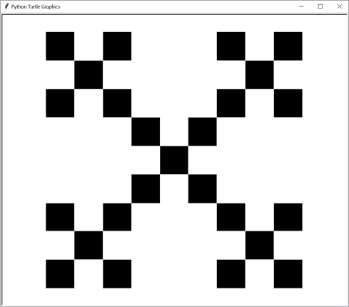
Figure 9-20: A box fractal, drawn to two levels
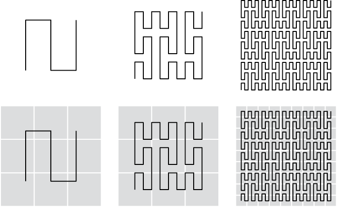
Figure 9-21: The first three iterations of the Peano curve, from left to right. The bottom row includes the 3 × 3 sections that each part of the curve is split across.