Check out other books by Al Sweigart, free online or available for purchase:


...and other books as well! Or register for the online video course. You can also donate to support the author directly.


Divide-and-conquer algorithms are those that split large problems into smaller subproblems, then divide those subproblems into ones that are smaller yet, until they become trivial to conquer. This approach makes recursion an ideal technique to use: the recursive case divides the problem into self-similar subproblems, and the base case occurs when the subproblem has been reduced to a trivial size. One benefit of this approach is that these problems can be worked on in parallel, allowing multiple central processing unit (CPU) cores or computers to work on them.
In this chapter, we’ll look at some common algorithms that use recursion to divide and conquer, such as binary search, quicksort, and merge sort. We’ll also reexamine summing an array of integers, this time with a divide-and-conquer approach. Finally, we’ll take a look at the more esoteric Karatsuba multiplication algorithm, developed in 1960, that laid the basis for computer hardware’s fast integer multiplication.
Let’s say you have a bookshelf of 100 books. You can’t remember which books you have or their exact locations on the shelf, but you do know that they are sorted alphabetically by title. To find your book Zebras: The Complete Guide, you wouldn’t start at the beginning of the bookshelf, where Aaron Burr Biography is, but rather toward the end of the bookshelf. Your zebra book wouldn’t be the very last book on the shelf if you also had books on zephyrs, zoos, and zygotes, but it would be close. Thus, you can use the facts that the books are in alphabetical order and that Z is the last letter of the alphabet as heuristics, or approximate clues, to look toward the end of the shelf rather than the beginning.
Binary search is a technique for locating a target item in a sorted list by repeatedly determining which half of the list the item is in. The most impartial way to search the bookshelf is to start with a book in the middle, and then ascertain if the target book you’re looking for is in the left half or the right half.
You can then repeat this process, as shown in Figure 5-1: look at the book in the middle of your chosen half and then determine whether your target book is in the left-side quarter or the right-side quarter. You can do this until you either find the book, or find the place where the book should be but isn’t and declare that the book doesn’t exist on the shelf.
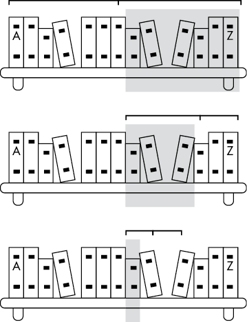
Figure 5-1: A binary search repeatedly determines which half of a range contains your target item in a sorted array of items.
This process scales efficiently; doubling the number of books to search adds only one step to the search process. A linear search of a shelf with 50 books takes 50 steps, and a linear search of a shelf with 100 books takes 100 steps. But a binary search of a shelf with 50 books takes only 6 steps, and a shelf with 100 books takes only 7 steps.
Let’s ask the three recursion questions about our binary search implementation:
left > right.)Examine the following binarySearch() function in our binarySearch.py program, which locates a value, needle, in a sorted list of values, haystack:
Python
def binarySearch(needle, haystack, left=None, right=None):
    # By default, `left` and `right` are all of `haystack`:
    if left is None:
        left = 0 # `left` defaults to the 0 index.
    if right is None:
        right = len(haystack) - 1 # `right` defaults to the last index.

    print('Searching:', haystack[left:right + 1])

    if left > right: # BASE CASE
         return None # The `needle` is not in `haystack`.

    mid = (left + right) // 2
    if needle == haystack[mid]: # BASE CASE
         return mid # The `needle` has been found in `haystack`
    elif needle < haystack[mid]: # RECURSIVE CASE
         return binarySearch(needle, haystack, left, mid - 1)
    elif needle > haystack[mid]: # RECURSIVE CASE
         return binarySearch(needle, haystack, mid + 1, right)

print(binarySearch(13, [1, 4, 8, 11, 13, 16, 19, 19]))
The binarySearch.html program has this JavaScript equivalent:
JavaScript
<script type="text/javascript">
function binarySearch(needle, haystack, left, right) {
    // By default, `left` and `right` are all of `haystack`:
    if (left === undefined) {
        left = 0; // `left` defaults to the 0 index.
    }
    if (right === undefined) {
        right = haystack.length - 1; // `right` defaults to the last index.
    }

    document.write("Searching: [" +
    haystack.slice(left, right + 1).join(", ") + "]<br />");

    if (left > right) { // BASE CASE
         return null; // The `needle` is not in `haystack`.
    }

    let mid = Math.floor((left + right) / 2);
    if (needle == haystack[mid]) { // BASE CASE
         return mid; // The `needle` has been found in `haystack`.
    } else if (needle < haystack[mid]) { // RECURSIVE CASE
         return binarySearch(needle, haystack, left, mid - 1);
    } else if (needle > haystack[mid]) { // RECURSIVE CASE
         return binarySearch(needle, haystack, mid + 1, right);
    }
}

document.write(binarySearch(13, [1, 4, 8, 11, 13, 16, 19, 19]));
</script>
When you run these programs, the list [1, 4, 8, 11, 13, 16, 19, 19] is searched for 13, and the output looks like this:
Searching: [1, 4, 8, 11, 13, 16, 19, 19]
Searching: [13, 16, 19, 19]
Searching: [13]
4
The target value 13 is indeed at index 4 in that list.
The code calculates the middle index (stored in mid) of the range defined by the left and right indices. At first, this range is the entire length of the items list. If the value at the mid index is the same as needle, then mid is returned. Otherwise, we need to figure out whether our target value is in the left half of the range (in which case, the new range to search is left to mid - 1) or in the right half (in which case, the new range to search is mid + 1 to end).
We already have a function that can search this new range: binarySearch() itself! A recursive call is made on the new range. If we ever get to the point where the right end of the search range comes before the left, we know that our search range has shrunk down to zero and our target value isn’t to be found.
Notice that the code performs no actions after the recursive call returns; it immediately returns the return value of the recursive function call. This feature means that we could implement tail call optimization for this recursive algorithm, a practice we explain in Chapter 8. But also, it means that binary search can easily be implemented as an iterative algorithm that doesn’t use recursive function calls. This book’s downloadable resources at https://nostarch.com/recursive-book-recursion include the source code for an iterative binary search for you to compare with the recursive binary search.
Remember that binarySearch()’s speed advantage comes from the fact that the values in items are sorted. If the values are out of order, the algorithm won’t work. Enter quicksort, a recursive sorting algorithm developed by computer scientist Tony Hoare in 1959.
Quicksort uses a divide-and-conquer technique called partitioning. Think of partitioning this way: imagine you have a large pile of unalphabetized books. Grabbing one book and placing it in the right spot on the shelf means you’ll spend a lot of time rearranging the bookshelf as it gets full. It would help if you first turned the pile of books into two piles: an A to M pile and an N to Z pile. (In this example, M would be our pivot.)
You haven’t sorted the pile, but you have partitioned it. And partitioning is easy: the book doesn’t have to go into the correct place in one of the two piles, it just has to go into the correct pile. Then you can further partition these two piles into four piles: A to G, H to M, N to T, and U to Z. This is shown in Figure 5-2. If you keep partitioning, you end up with piles that contain one book each (the base case), and the piles are now in sorted order. This means the books are now in sorted order as well. This repeated partitioning is how quicksort works.
For the first partitioning of A to Z, we select M as the pivot value because it’s the middle letter between A and Z. However, if our collection of books consisted of one book about Aaron Burr and 99 books about zebras, zephyrs, zoos, zygotes, and other Z topics, our two partitioned piles would be heavily unbalanced. We would have the single Aaron Burr book in the A to M pile and every other book in the M to Z pile. The quicksort algorithm works fastest when the partitions are evenly balanced, so selecting a good pivot value at each partition step is important.
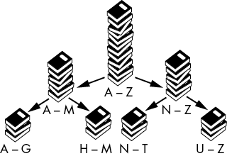
Figure 5-2: Quicksort works by repeatedly partitioning items into two sets.
However, if you don’t know anything about the data you’re sorting, it’s impossible to select an ideal pivot. This is why the generic quicksort algorithm simply uses the last value in the range for the pivot value.
In our implementation, each call to quicksort() is given an array of items to sort. It is also given left and right arguments specifying the range of indices in that array to sort, similar to binarySearch()’s left and right arguments. The algorithm selects a pivot value to compare with the other values in the range, then places the values to either the left side of the range (if they’re less than the pivot value) or the right side (if they’re greater than the pivot value). This is the partition step. Next, the quicksort() function is recursively called on these two, smaller ranges until a range has been reduced to zero. The list becomes more and more sorted as the recursive calls are made, until finally the entire list is in the correct order.
Note that the algorithm modifies the array in place. See “Modifying a List or Array in Place” in Chapter 4 for details. Thus, the quicksort() function doesn’t return a sorted array. The base case merely returns to stop producing more recursive calls.
Let’s ask the three recursion questions about our binary search implementation:
The following quicksort() function in the quicksort.py Python program sorts the values in the items list into ascending order:
def quicksort(items, left=None, right=None):
    # By default, `left` and `right` span the entire range of `items`:
    if left is None:
        left = 0 # `left` defaults to the 0 index.
    if right is None:
        right = len(items) - 1 # `right` defaults to the last index.

    print('\nquicksort() called on this range:', items[left:right + 1])
    print('................The full list is:', items)

    if right <= left: ❶
        # With only zero or one item, `items` is already sorted.
        return  # BASE CASE

    # START OF THE PARTITIONING
    i = left # i starts at the left end of the range. ❷
    pivotValue = items[right] # Select the last value for the pivot.

    print('....................The pivot is:', pivotValue)

    # Iterate up to, but not including, the pivot:
    for j in range(left, right):
        # If a value is less than the pivot, swap it so that it's on the
        # left side of `items`:
        if items[j] <= pivotValue:
            # Swap these two values:
            items[i], items[j] = items[j], items[i] ❸
            i += 1

    # Put the pivot on the left side of `items`:
    items[i], items[right] = items[right], items[i]
    # END OF THE PARTITIONING

    print('....After swapping, the range is:', items[left:right + 1])
    print('Recursively calling quicksort on:', items[left:i], 'and', items[i + 1:right + 1])

    # Call quicksort() on the two partitions:
    quicksort(items, left, i - 1)   # RECURSIVE CASE
    quicksort(items, i + 1, right)  # RECURSIVE CASE

myList = [0, 7, 6, 3, 1, 2, 5, 4]
quicksort(myList)
print(myList)
The quicksort.html program contains the JavaScript equivalent:
<script type="text/javascript">
function quicksort(items, left, right) {
    // By default, `left` and `right` span the entire range of `items`:
    if (left === undefined) {
        left = 0; // `left` defaults to the 0 index.
    }
    if (right === undefined) {
        right = items.length - 1; // `right` defaults to the last index.
    }

    document.write("<br /><pre>quicksort() called on this range: [" +
    items.slice(left, right + 1).join(", ") + "]</pre>");
    document.write("<pre>................The full list is: [" + items.join(", ") + "]</pre>");

    if (right <= left) { ❶
        // With only zero or one item, `items` is already sorted.
        return; // BASE CASE
    }

    // START OF THE PARTITIONING
    let i = left; ❷ // i starts at the left end of the range.
    let pivotValue = items[right]; // Select the last value for the pivot.

    document.write("<pre>....................The pivot is: " + pivotValue.toString() +
"</pre>");

    // Iterate up to, but not including, the pivot:
    for (let j = left; j < right; j++) {
        // If a value is less than the pivot, swap it so that it's on the
        // left side of `items`:
        if (items[j] <= pivotValue) {
            // Swap these two values:
            [items[i], items[j]] = [items[j], items[i]]; ❸
            i++;
        }
    }

    // Put the pivot on the left side of `items`:
    [items[i], items[right]] = [items[right], items[i]];
    // END OF THE PARTITIONING

    document.write("<pre>....After swapping, the range is: [" + items.slice(left, right + 1).join(", ") + "]</pre>");
    document.write("<pre>Recursively calling quicksort on: [" + items.slice(left, i).join(", ") + "] and [" + items.slice(i + 1, right + 1).join(", ") + "]</pre>");

    // Call quicksort() on the two partitions:
    quicksort(items, left, i - 1); // RECURSIVE CASE
    quicksort(items, i + 1, right); // RECURSIVE CASE
}

let myList = [0, 7, 6, 3, 1, 2, 5, 4];
quicksort(myList);
document.write("<pre>[" + myList.join(", ") + "]</pre>");
</script>
This code is similar to the code in the binary search algorithm. As defaults, we set the left and right ends of the range within the items array to the beginning and end of the entire array. If the algorithm reaches the base case of the right end at or before the left end (a range of one or zero items), the sorting is finished ❶.
In each call to quicksort(), we partition the items in the current range (defined by the indices in left and right), and then swap them around so that the items less than the pivot value end up on the left side of the range and the items greater than the pivot value end up on the right side of the range. For example, if 42 is the pivot value in the array [81, 48, 94, 87, 83, 14, 6, 42], a partitioned array would be [14, 6, 42, 81, 48, 94, 87, 83]. Note that a partitioned array is not the same thing as a sorted one: although the two items to the left of 42 are less than 42, and the five items to the right of 42 are greater than 42, the items are not in sorted order.
The bulk of the quicksort() function is the partitioning step. To get an idea of how partitioning works, imagine an index j that begins at the left end of the range and moves to the right end ❷. We compare the item at index j with the pivot value and then move right to compare the next item. The pivot value can be arbitrarily chosen from any value in the range, but we’ll always use the value at the right end of the range.
Imagine a second index i that also begins at the left end. If the item at index j is less than or equal to the pivot, the items at indices i and j are swapped ❸ and i is increased to the next index. So while j always increases (that is, moves right) after each comparison with the pivot value, i increases only if the item at index j is less than or equal to the pivot.
The names i and j are commonly used for variables that hold array indices. Someone else’s quicksort() implementation may instead use j and i, or even completely different variables. The important thing to remember is that two variables store indices and behave as shown here.
As an example, let’s work through the first partitioning of the array [0, 7, 6, 3, 1, 2, 5, 4], and the range defined by left of 0 and right of 7 to cover the full size of the array. The pivot will be the value at the right end, 4. The i and j index begin at index 0, the left end of the range. At each step, index j always moves to the right. Index i moves only if the value at index j is less than or equal to the pivot value. The items array, the i index, and the j index begin as follows:
items:   [0, 7, 6, 3, 1, 2, 5, 4]
indices:  0  1  2  3  4  5  6  7
          ^
i = 0     i
j = 0     j
The value at index j (which is 0) is less than or equal to the pivot value (which is 4), so swap the values at i and j. This results in no actual change since i and j are the same index. Also, increase i so that it moves to the right. The j index increases for every comparison with the pivot value. The state of the variables now looks like this:
items:   [0, 7, 6, 3, 1, 2, 5, 4]
indices:  0  1  2  3  4  5  6  7
             ^
i = 1        i
j = 1        j
The value at index j (which is 7) is not less than or equal to the pivot value (which is 4), so don’t swap the values. Remember, j always increases, but i increases only after a swap is performed—so i is always either at or to the left of j. The state of the variables now looks like this:
items:   [0, 7, 6, 3, 1, 2, 5, 4]
indices:  0  1  2  3  4  5  6  7
             ^
i = 1        i  ^
j = 2           j
The value at index j (which is 6) is not less than or equal to the pivot value (which is 4), so don’t swap the values. The state of the variables now looks like this:
items:   [0, 7, 6, 3, 1, 2, 5, 4]
indices:  0  1  2  3  4  5  6  7
             ^
i = 1        i     ^
j = 3              j
The value at index j (which is 3) is less than or equal to the pivot value (which is 4), so swap the values at i and j. The 7 and 3 swap positions. Also, increase i so that it moves to the right. The state of the variables now looks like this:
items:   [0, 3, 6, 7, 1, 2, 5, 4]
indices:  0  1  2  3  4  5  6  7
                ^
i = 2           i     ^
j = 4                 j
The value at index j (which is 1) is less than or equal to the pivot value (which is 4), so swap the values at i and j. The 6 and 1 swap positions. Also, increase i so that it moves to the right. The state of the variables now looks like this:
items:   [0, 3, 1, 7, 6, 2, 5, 4]
indices:  0  1  2  3  4  5  6  7
                   ^
i = 3              i     ^
j = 5                    j
The value at index j (which is 2) is less than or equal to the pivot value (which is 4), so swap the values at i and j. The 7 and 2 swap positions. Also, increase i so that it moves to the right. The state of the variables now looks like this:
items:   [0, 3, 1, 2, 6, 7, 5, 4]
indices:  0  1  2  3  4  5  6  7
                      ^
i = 4                 i     ^
j = 6                       j
The value at index j (which is 6) is not less than or equal to the pivot value (which is 4), so don’t swap the values. The state of the variables now looks like this:
items:   [0, 3, 1, 2, 6, 7, 5, 4]
indices:  0  1  2  3  4  5  6  7
                      ^
i = 4                 i        ^
j = 7                          j
We’ve reached the end of the partitioning. The index j is at the pivot value (which is always the rightmost value in the range), so let’s swap i and j one last time to make sure the pivot is not on the right half of the partition. The 6 and 4 swap positions. The state of the variables now looks like this:
items:   [0, 3, 1, 2, 4, 7, 5, 6]
indices:  0  1  2  3  4  5  6  7
                      ^
i = 4                 i        ^
j = 7                          j
Notice what is happening with the i index: this index will always receive the values smaller than the pivot value as a result of swapping; then the i index moves right to receive future smaller-than-the-pivot values. As a result, everything to the left of the i index is smaller than or equal to the pivot, and everything to the right of the i index is greater than the pivot.
The entire process repeats as we recursively call quicksort() on the left and right partitions. When we partition these two halves (and then partition the four halves of these two halves with more recursive quicksort() calls, and so on), the entire array ends up sorted.
When we run these programs, the output shows the process of sorting the [0, 7, 6, 3, 1, 2, 5, 4] list. The rows of periods are meant to help you line up the output when writing the code:
quicksort() called on this range: [0, 7, 6, 3, 1, 2, 5, 4]
................The full list is: [0, 7, 6, 3, 1, 2, 5, 4]
....................The pivot is: 4
....After swapping, the range is: [0, 3, 1, 2, 4, 7, 5, 6]
Recursively calling quicksort on: [0, 3, 1, 2] and [7, 5, 6]

quicksort() called on this range: [0, 3, 1, 2]
................The full list is: [0, 3, 1, 2, 4, 7, 5, 6]
....................The pivot is: 2
....After swapping, the range is: [0, 1, 2, 3]
Recursively calling quicksort on: [0, 1] and [3]

quicksort() called on this range: [0, 1]
................The full list is: [0, 1, 2, 3, 4, 7, 5, 6]
....................The pivot is: 1
....After swapping, the range is: [0, 1]
Recursively calling quicksort on: [0] and []

quicksort() called on this range: [0]
................The full list is: [0, 1, 2, 3, 4, 7, 5, 6]

quicksort() called on this range: []
................The full list is: [0, 1, 2, 3, 4, 7, 5, 6]

quicksort() called on this range: [3]
................The full list is: [0, 1, 2, 3, 4, 7, 5, 6]

quicksort() called on this range: [7, 5, 6]
................The full list is: [0, 1, 2, 3, 4, 7, 5, 6]
....................The pivot is: 6
....After swapping, the range is: [5, 6, 7]
Recursively calling quicksort on: [5] and [7]

quicksort() called on this range: [5]
................The full list is: [0, 1, 2, 3, 4, 5, 6, 7]

quicksort() called on this range: [7]
................The full list is: [0, 1, 2, 3, 4, 5, 6, 7]

Sorted: [0, 1, 2, 3, 4, 5, 6, 7]
Quicksort is a commonly used sorting algorithm because it is straightforward to implement and, well, quick. The other commonly used sorting algorithm, merge sort, is also fast and uses recursion. We cover it next.
Computer scientist John von Neumann developed merge sort in 1945. It uses a divide-merge approach: each recursive call to mergeSort() divides the unsorted list into halves until they’ve been whittled down into lists of lengths of zero or one. Then, as the recursive calls return, these smaller lists are merged together into sorted order. When the last recursive call has returned, the entire list will have been sorted.
For example, the divide step takes a list, such as [2, 9, 8, 5, 3, 4, 7, 6], and splits it into two lists, like [2, 9, 8, 5] and [3, 4, 7, 6], to pass to two recursive function calls. At the base case, the lists have been divided into lists of zero or one item. A list with nothing or one item is naturally sorted. After the recursive calls return, the code merges these small, sorted lists together into larger sorted lists until finally the entire list is sorted. Figure 5-3 shows an example using merge sort on playing cards.
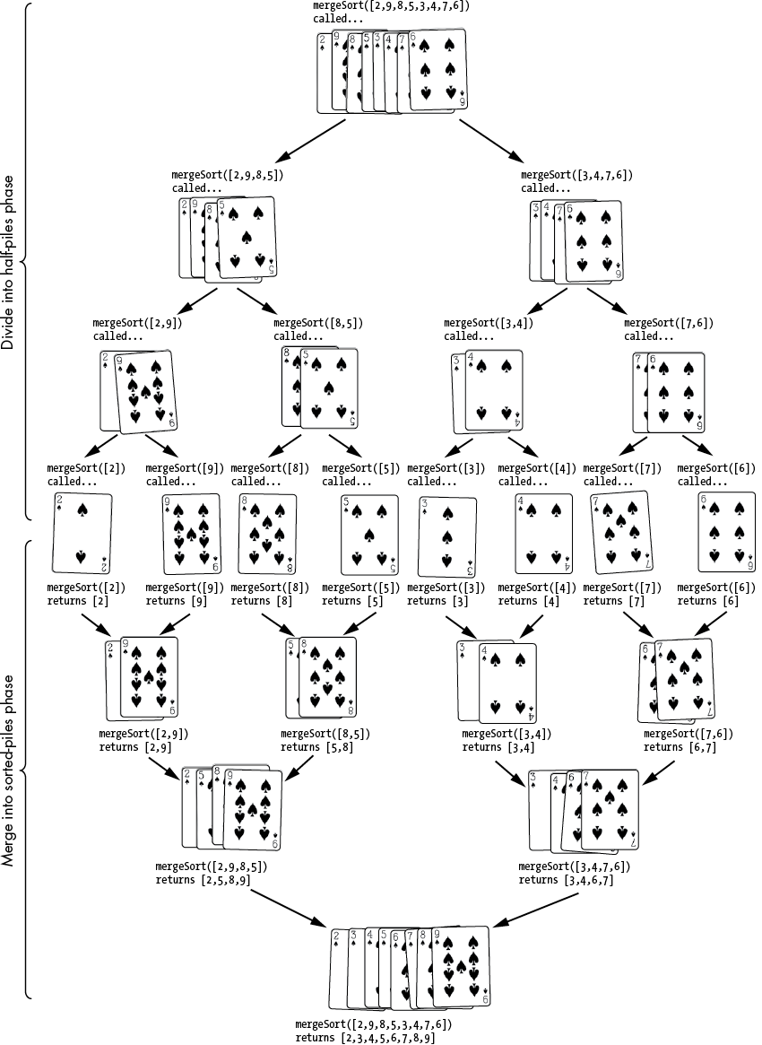
Figure 5-3: The divide and merge phases of merge sort
For example, at the end of the division phase, we have eight separate lists of single numbers: [2], [9], [8], [5], [3], [4], [7], [6]. A list of just one number is naturally in sorted order. Merging two sorted lists into a larger sorted list involves looking at the start of both smaller lists and appending the smaller value to the larger list. Figure 5-4 shows an example of merging [2, 9] and [5, 8]. This is repeatedly done in the merge phase until the end result is that the original mergeSort() call returns the full list in sorted order.
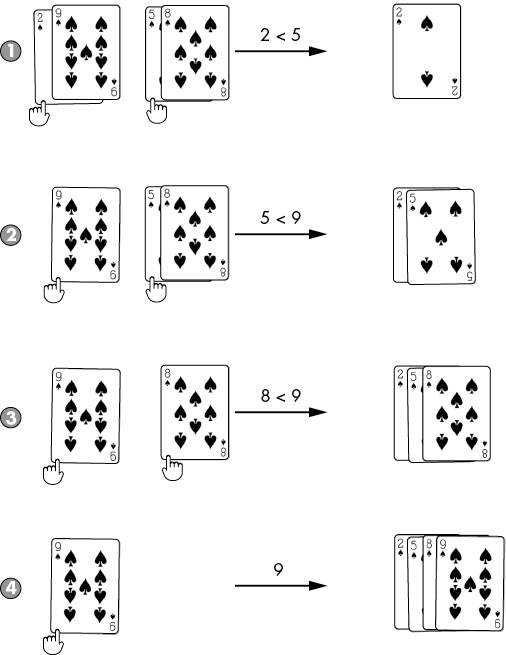
Figure 5-4: The merge step compares the two values at the start of the smaller sorted lists and moves them to the larger sorted list. Merging four cards requires only four steps.
Let’s ask our three recursive algorithm questions about the merge sort algorithm:
The following mergeSort() function in the mergeSort.py Python program sorts the values in the items list into ascending order:
import math

def mergeSort(items):
    print('.....mergeSort() called on:', items)

    # BASE CASE - Zero or one item is naturally sorted:
    if len(items) == 0 or len(items) == 1:
        return items ❶

    # RECURSIVE CASE - Pass the left and right halves to mergeSort():
    # Round down if items doesn't divide in half evenly:
    iMiddle = math.floor(len(items) / 2) ❷

    print('................Split into:', items[:iMiddle], 'and', items[iMiddle:])

    left = mergeSort(items[:iMiddle]) ❸
    right = mergeSort(items[iMiddle:])

    # BASE CASE - Returned merged, sorted data:
    # At this point, left should be sorted and right should be
    # sorted. We can merge them into a single sorted list.
    sortedResult = []
    iLeft = 0
    iRight = 0
    while (len(sortedResult) < len(items)):
        # Append the smaller value to sortedResult.
        if left[iLeft] < right[iRight]: ❹
            sortedResult.append(left[iLeft])
            iLeft += 1
        else:
            sortedResult.append(right[iRight])
            iRight += 1

        # If one of the pointers has reached the end of its list,
        # put the rest of the other list into sortedResult.
        if iLeft == len(left):
            sortedResult.extend(right[iRight:])
            break
        elif iRight == len(right):
            sortedResult.extend(left[iLeft:])
            break

    print('The two halves merged into:', sortedResult)

    return sortedResult # Returns a sorted version of items.

myList = [2, 9, 8, 5, 3, 4, 7, 6]
myList = mergeSort(myList)
print(myList)
The mergeSort.html program contains the equivalent JavaScript program:
<script type="text/javascript">
function mergeSort(items) {
    document.write("<pre>" + ".....mergeSort() called on: [" +
    items.join(", ") + "]</pre>");

    // BASE CASE - Zero or one item is naturally sorted:
    if (items.length === 0 || items.length === 1) { // BASE CASE
        return items; ❶
    }

    // RECURSIVE CASE - Pass the left and right halves to mergeSort():
    // Round down if items doesn't divide in half evenly:
    let iMiddle = Math.floor(items.length / 2); ❷

    document.write("<pre>................Split into: [" + items.slice(0, iMiddle).join(", ") +
    "] and [" + items.slice(iMiddle).join(", ") + "]</pre>");

    let left = mergeSort(items.slice(0, iMiddle)); ❸
    let right = mergeSort(items.slice(iMiddle));

    // BASE CASE - Returned merged, sorted data:
    // At this point, left should be sorted and right should be
    // sorted. We can merge them into a single sorted list.
    let sortedResult = [];
    let iLeft = 0;
    let iRight = 0;
    while (sortedResult.length < items.length) {
        // Append the smaller value to sortedResult.
        if (left[iLeft] < right[iRight]) { ❹
            sortedResult.push(left[iLeft]);
            iLeft++;
        } else {
            sortedResult.push(right[iRight]);
            iRight++;
        }

        // If one of the pointers has reached the end of its list,
        // put the rest of the other list into sortedResult.
        if (iLeft == left.length) {
            Array.prototype.push.apply(sortedResult, right.slice(iRight));
            break;
        } else if (iRight == right.length) {
            Array.prototype.push.apply(sortedResult, left.slice(iLeft));
            break;
        }
    }

    document.write("<pre>The two halves merged into: [" + sortedResult.join(", ") +
    "]</pre>");

    return sortedResult; // Returns a sorted version of items.
}

let myList = [2, 9, 8, 5, 3, 4, 7, 6];
myList = mergeSort(myList);
document.write("<pre>[" + myList.join(", ") + "]</pre>");
</script>
The mergeSort() function (and all the recursive calls to the mergeSort() function) takes an unsorted list and returns a sorted list. The first step in this function is to check for the base case of a list containing only zero or one item ❶. This list is already sorted, so the function returns the list as is.
Otherwise, the function determines the middle index of the list ❷ so that we know where to split it into the left- and right-half lists to pass to two recursive function calls ❸. The recursive function calls return sorted lists, which we store in the left and right variables.
The next step is to merge these two sorted half lists into one sorted full list named sortedResult. We’ll maintain two indices for the left and right lists named iLeft and iRight. Inside a loop, the smaller of the two values ❹ is appended to sortedResult, and its respective index variable (either iLeft or iRight) is incremented. If either iLeft or iRight reaches the end of its list, the remaining items in the other half’s list are appended to sortedResult.
Let’s follow an example of the merging step if the recursive calls have returned [2, 9] for left and [5, 8] for right. Since these lists were returned from mergeSort() calls, we can always assume they are sorted. We must merge them into a single sorted list in sortedResult for the current mergeSort() call to return to its caller.
The iLeft and iRight indices begin at 0. We compare the value at left[iLeft] (which is 2) and right[iRight] (which is 5) to find the smaller one:
sortedResult = []
      left: [2, 9]    right: [5, 8]
   indices:  0  1             0  1
 iLeft = 0   ^
iRight = 0                    ^
Since left[iLeft]’s value, 2, is the smaller of the values, we append it to sortedResult and increase iLeft from 0 to 1. The state of the variables is now as follows:
sortedResult = [2]
      left: [2, 9]    right: [5, 8]
   indices:  0  1             0  1
 iLeft = 1      ^
iRight = 0                    ^
Comparing left[iLeft] and right[iRight] again, we find that of 9 and 5, right[iRight]’s 5 is smaller. The code appends the 5 to sortedResult and increases iRight from 0 to 1. The state of the variables is now the following:
sortedResult = [2, 5]
      left: [2, 9]    right: [5, 8]
   indices:  0  1             0  1
 iLeft = 1      ^
iRight = 1                       ^
Comparing left[iLeft] and right[iRight] again, we find that, of 9 and 8, right[iRight]’s 8 is smaller. The code appends the 8 to sortedResult and increases iRight from 0 to 1. Here’s the state of the variables now:
sortedResult = [2, 5, 8]
      left: [2, 9]    right: [5, 8]
   indices:  0  1             0  1
 iLeft = 1      ^
iRight = 2                         ^
Because iRight is now 2 and equal to the length of the right list, the remaining items in left from the iLeft index to the end are appended to sortedResult, as no more items remain in right to compare them to. This leaves sortedResult as [2, 5, 8, 9], the sorted list it needs to return. This merging step is performed for every call to mergeSort() to produce the final sorted list.
When we run the mergeSort.py and mergeSort.html programs, the output shows the process of sorting the [2, 9, 8, 5, 3, 4, 7, 6] list:
.....mergeSort() called on: [2, 9, 8, 5, 3, 4, 7, 6]
................Split into: [2, 9, 8, 5] and [3, 4, 7, 6]
.....mergeSort() called on: [2, 9, 8, 5]
................Split into: [2, 9] and [8, 5]
.....mergeSort() called on: [2, 9]
................Split into: [2] and [9]
.....mergeSort() called on: [2]
.....mergeSort() called on: [9]
The two halves merged into: [2, 9]
.....mergeSort() called on: [8, 5]
................Split into: [8] and [5]
.....mergeSort() called on: [8]
.....mergeSort() called on: [5]
The two halves merged into: [5, 8]
The two halves merged into: [2, 5, 8, 9]
.....mergeSort() called on: [3, 4, 7, 6]
................Split into: [3, 4] and [7, 6]
.....mergeSort() called on: [3, 4]
................Split into: [3] and [4]
.....mergeSort() called on: [3]
.....mergeSort() called on: [4]
The two halves merged into: [3, 4]
.....mergeSort() called on: [7, 6]
................Split into: [7] and [6]
.....mergeSort() called on: [7]
.....mergeSort() called on: [6]
The two halves merged into: [6, 7]
The two halves merged into: [3, 4, 6, 7]
The two halves merged into: [2, 3, 4, 5, 6, 7, 8, 9]
[2, 3, 4, 5, 6, 7, 8, 9]
As you can see from the output, the function divides the [2, 9, 8, 5, 3, 4, 7, 6] list into [2, 9, 8, 5] and [3, 4, 7, 6] and passes these to recursive mergeSort() calls. The first list is further split into [2, 9] and [8, 5]. That [2, 9] list is split into [2] and [9]. These single-value lists cannot be divided anymore, so we have reached our base case. These lists are merged back into sorted order as [2, 9]. The function divides the [8, 5] list into [8] and [5], reaches the base case, and then merges back into [5, 8].
The [2, 9] and [5, 8] lists are individually in sorted order. Remember, mergeSort() doesn’t simply concatenate the lists into [2, 9, 5, 8], which would not be in sorted order. Rather, the function merges them into the sorted list [2, 5, 8, 9]. By the time the original mergeSort() call returns, the full list it returns is completely sorted.
We already covered summing an array of integers in Chapter 3 with the head-tail technique. In this chapter, we’ll use a divide-and-conquer strategy. Since the associative property of addition means that adding 1 + 2 + 3 + 4 is the same as adding the sums of 1 + 2 and 3 + 4, we can divide a large array of numbers to sum into two smaller arrays of numbers to sum.
The benefit is that for larger sets of data to process, we could farm out the subproblems to different computers and have them all work together in parallel. There’s no need to wait for the first half of the array to be summed before another computer can start summing the second half. This is a large advantage of the divide-and-conquer technique, as CPUs aren’t getting much faster but we can have multiple CPUs work simultaneously.
Let’s ask the three questions about recursive algorithms for our summation function:
0) or an array containing one number (where we return the number).The sumDivConq.py Python program implements the divide-and-conquer strategy for adding numbers in the sumDivConq() function:
Python
def sumDivConq(numbers):
    if len(numbers) == 0: # BASE CASE
      ❶ return 0
    elif len(numbers) == 1: # BASE CASE
      ❷ return numbers[0]
    else: # RECURSIVE CASE
      ❸ mid = len(numbers) // 2
        leftHalfSum = sumDivConq(numbers[0:mid])
        rightHalfSum = sumDivConq(numbers[mid:len(numbers) + 1])
      ❹ return leftHalfSum + rightHalfSum

nums = [1, 2, 3, 4, 5]
print('The sum of', nums, 'is', sumDivConq(nums))
nums = [5, 2, 4, 8]
print('The sum of', nums, 'is', sumDivConq(nums))
nums = [1, 10, 100, 1000]
print('The sum of', nums, 'is', sumDivConq(nums))
The sumDivConq.html program contains the JavaScript equivalent:
JavaScript
<script type="text/javascript">
function sumDivConq(numbers) {
    if (numbers.length === 0) { // BASE CASE
      ❶ return 0;
    } else if (numbers.length === 1) { // BASE CASE
      ❷ return numbers[0];
    } else { // RECURSIVE CASE
      ❸ let mid = Math.floor(numbers.length / 2);
        let leftHalfSum = sumDivConq(numbers.slice(0, mid));
        let rightHalfSum = sumDivConq(numbers.slice(mid, numbers.length + 1));
      ❹ return leftHalfSum + rightHalfSum;
    }
}

let nums = [1, 2, 3, 4, 5];
document.write('The sum of ' + nums + ' is ' + sumDivConq(nums) + "<br />");
nums = [5, 2, 4, 8];
document.write('The sum of ' + nums + ' is ' + sumDivConq(nums) + "<br />");
nums = [1, 10, 100, 1000];
document.write('The sum of ' + nums + ' is ' + sumDivConq(nums) + "<br />");
</script>
The output of this program is:
The sum of [1, 2, 3, 4, 5] is 15
The sum of [5, 2, 4, 8] is 19
The sum of [1, 10, 100, 1000] is 1111
The sumDivConq() function first checks the numbers array for having either zero or one number in it. These trivial base cases are easy to sum since they require no addition: return either 0 ❶ or the lone number in the array ❷. Everything else is a recursive case; the middle index of the array is calculated ❸ so that separate recursive calls with the left half and right half of the numbers array are made. The sum of these two return values becomes the return value for the current sumDivConq() call ❹.
Because of the associative nature of addition, there’s no reason an array of numbers must be added sequentially by a single computer. Our program carries out all operations on the same computer, but for large arrays or calculations more complicated than addition, our program could send the halves to other computers to complete. The problem can be divided into similar subproblems, which is a huge hint that a recursive approach can be taken.
The * operator makes multiplication easy to do in high-level programming languages such as Python and JavaScript. But low-level hardware needs a way to perform multiplication using more primitive operations. We could multiply two integers using only addition with a loop, such as in the following Python code to multiply 5678 * 1234:
>>> x = 5678
>>> y = 1234
>>> product = 0
>>> for i in range(x):
...     product += y
...
>>> product
7006652
However, this code doesn’t scale efficiently for large integers. Karatsuba multiplication is a fast, recursive algorithm discovered in 1960 by Anatoly Karatsuba that can multiply integers using addition, subtraction, and a precomputed multiplication table of all products from single-digit numbers. This multiplication table, shown in Figure 5-5, is called a lookup table.
Our algorithm won’t need to multiply single-digit numbers because it can just look them up in the table. By using memory to store precomputed values, we increase memory usage to decrease CPU runtime.
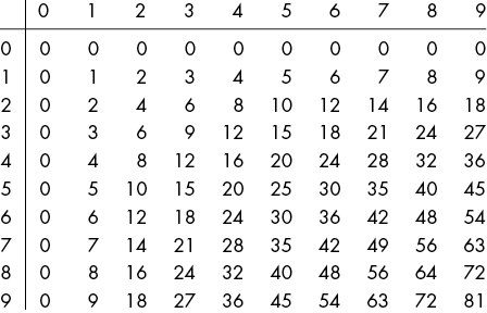
Figure 5-5: A lookup table, such as this table of products of all single-digit numbers, saves our program from repeat calculations as the computer stores the precomputed values in memory for later retrieval.
We’ll implement Karatsuba multiplication in a high-level language like Python or JavaScript as though the * operator didn’t already exist. Our karatsuba() function accepts two integer arguments, x and y, to multiply. The Karatsuba algorithm has five steps, and the first three involve making recursive calls to karatsuba() with arguments that are smaller, broken-down integers derived from x and y. The base case occurs when the x and y arguments are both single-digit numbers, in which case the product can be found in the precomputed lookup table.
We also define four more variables: a and b are each half of the digits of x, and c and d are each half of the digits of y, as shown in Figure 5-6. For example, if x and y are 5678 and 1234, respectively, then a is 56, b is 78, c is 12, and d is 34.

Figure 5-6: The integers to multiply, x and y, are divided into halves a, b, c, and d.
Here are the five steps of the Karatsuba algorithm:
a and c either from the multiplication lookup table or from a recursive call to karatsuba().b and d either from the multiplication lookup table or from a recursive call to karatsuba().a + c and b + d either from the multiplication lookup table or from a recursive call to karatsuba().The result of step 5 is the product of x and y. The specifics of how to pad the step 1 and step 4 results with zeros are explained later in this section.
Let’s ask our three recursive algorithm questions about the karatsuba() function:
a, b, c, and d values derived from the x and y arguments.a, b, c, and d are each half of the digits of x and y and themselves are used for the next recursive call’s x and y arguments, the recursive call’s arguments become closer and closer to the single-digit numbers the base case requires.Our Python implementation for Karatsuba multiplication is in the karatsubaMultiplication.py program:
import math

# Create a lookup table of all single-digit multiplication products:
MULT_TABLE = {} ❶
for i in range(10):
    for j in range(10):
        MULT_TABLE[(i, j)] = i * j

def padZeros(numberString, numZeros, insertSide):
    """Return a string padded with zeros on the left or right side."""
    if insertSide == 'left':
        return '0' * numZeros + numberString
    elif insertSide == 'right':
        return numberString + '0' * numZeros

def karatsuba(x, y):
    """Multiply two integers with the Karatsuba algorithm. Note that
    the * operator isn't used anywhere in this function."""
    assert isinstance(x, int), 'x must be an integer'
    assert isinstance(y, int), 'y must be an integer'
    x = str(x)
    y = str(y)

    # At single digits, look up the products in the multiplication table:
    if len(x) == 1 and len(y) == 1: # BASE CASE
        print('Lookup', x, '*', y, '=', MULT_TABLE[(int(x), int(y))])
        return MULT_TABLE[(int(x), int(y))]

    # RECURSIVE CASE
    print('Multiplying', x, '*', y)

    # Pad with prepended zeros so that x and y are the same length:
    if len(x) < len(y): ❷
        # If x is shorter than y, pad x with zeros:
        x = padZeros(x, len(y) - len(x), 'left')
    elif len(y) < len(x):
        # If y is shorter than x, pad y with zeros:
        y = padZeros(y, len(x) - len(y), 'left')
    # At this point, x and y have the same length.

    halfOfDigits = math.floor(len(x) / 2) ❸

    # Split x into halves a & b, split y into halves c & d:
    a = int(x[:halfOfDigits])
    b = int(x[halfOfDigits:])
    c = int(y[:halfOfDigits])
    d = int(y[halfOfDigits:])

    # Make the recursive calls with these halves:
    step1Result = karatsuba(a, c) ❹ # Step 1: Multiply a & c.
    step2Result = karatsuba(b, d) # Step 2: Multiply b & d.
    step3Result = karatsuba(a + b, c + d) # Step 3: Multiply a + b & c + d.

    # Step 4: Calculate Step 3 - Step 2 - Step 1:
    step4Result = step3Result - step2Result - step1Result ❺

    # Step 5: Pad these numbers, then add them for the return value:
    step1Padding = (len(x) - halfOfDigits) + (len(x) - halfOfDigits)
    step1PaddedNum = int(padZeros(str(step1Result), step1Padding, 'right'))

    step4Padding = (len(x) - halfOfDigits)
    step4PaddedNum = int(padZeros(str(step4Result), step4Padding, 'right'))

    print('Solved', x, 'x', y, '=', step1PaddedNum + step2Result + step4PaddedNum)

    return step1PaddedNum + step2Result + step4PaddedNum ❻

# Example: 1357 x 2468 = 3349076
print('1357 * 2468 =', karatsuba(1357, 2468))
The JavaScript equivalent is in karatsubaMultiplication.html:
<script type="text/javascript">

// Create a lookup table of all single-digit multiplication products:
let MULT_TABLE = {}; ❶
for (let i = 0; i < 10; i++) {
    for (let j = 0; j < 10; j++) {
        MULT_TABLE[[i, j]] = i * j;
    }
}

function padZeros(numberString, numZeros, insertSide) {
    // Return a string padded with zeros on the left or right side.
    if (insertSide === "left") {
        return "0".repeat(numZeros) + numberString;
    } else if (insertSide === "right") {
        return numberString + "0".repeat(numZeros);
    }
}

function karatsuba(x, y) {
    // Multiply two integers with the Karatsuba algorithm. Note that
    // the * operator isn't used anywhere in this function.
    console.assert(Number.isInteger(x), "x must be an integer");
    console.assert(Number.isInteger(y), "y must be an integer");
    x = x.toString();
    y = y.toString();

    // At single digits, look up the products in the multiplication table:
    if ((x.length === 1) && (y.length === 1)) { // BASE CASE
        document.write("Lookup " + x.toString() + " * " + y.toString() + " = " +
        MULT_TABLE[[parseInt(x), parseInt(y)]] + "<br />");
        return MULT_TABLE[[parseInt(x), parseInt(y)]];
    }

    // RECURSIVE CASE
    document.write("Multiplying " + x.toString() + " * " + y.toString() +
    "<br />");

    // Pad with prepended zeros so that x and y are the same length:
    if (x.length < y.length) { ❷
        // If x is shorter than y, pad x with zeros:
        x = padZeros(x, y.length - x.length, "left");
    } else if (y.length < x.length) {
        // If y is shorter than x, pad y with zeros:
        y = padZeros(y, x.length - y.length, "left");
    }
    // At this point, x and y have the same length.

    let halfOfDigits = Math.floor(x.length / 2); ❸

    // Split x into halves a & b, split y into halves c & d:
    let a = parseInt(x.substring(0, halfOfDigits));
    let b = parseInt(x.substring(halfOfDigits));
    let c = parseInt(y.substring(0, halfOfDigits));
    let d = parseInt(y.substring(halfOfDigits));

    // Make the recursive calls with these halves:
    let step1Result = karatsuba(a, c); ❹ // Step 1: Multiply a & c.
    let step2Result = karatsuba(b, d); // Step 2: Multiply b & d.
    let step3Result = karatsuba(a + b, c + d); // Step 3: Multiply a + b & c + d.

    // Step 4: Calculate Step 3 - Step 2 - Step 1:
    let step4Result = step3Result - step2Result - step1Result; ❺

    // Step 5: Pad these numbers, then add them for the return value:
    let step1Padding = (x.length - halfOfDigits) + (x.length - halfOfDigits);
    let step1PaddedNum = parseInt(padZeros(step1Result.toString(), step1Padding, "right"));

    let step4Padding = (x.length - halfOfDigits);
    let step4PaddedNum = parseInt(padZeros((step4Result).toString(), step4Padding, "right"));

    document.write("Solved " + x + " x " + y + " = " +
    (step1PaddedNum + step2Result + step4PaddedNum).toString() + "<br />");

    return step1PaddedNum + step2Result + step4PaddedNum; ❻
}

// Example: 1357 x 2468 = 3349076
document.write("1357 * 2468 = " + karatsuba(1357, 2468).toString() + "<br />");
</script>
When you run this code, the output looks like this:
Multiplying 1357 * 2468
Multiplying 13 * 24
Lookup 1 * 2 = 2
Lookup 3 * 4 = 12
Lookup 4 * 6 = 24
Solved 13 * 24 = 312
Multiplying 57 * 68
Lookup 5 * 6 = 30
Lookup 7 * 8 = 56
Multiplying 12 * 14
Lookup 1 * 1 = 1
Lookup 2 * 4 = 8
Lookup 3 * 5 = 15
Solved 12 * 14 = 168
Solved 57 * 68 = 3876
Multiplying 70 * 92
Lookup 7 * 9 = 63
Lookup 0 * 2 = 0
Multiplying 7 * 11
Lookup 0 * 1 = 0
Lookup 7 * 1 = 7
Lookup 7 * 2 = 14
Solved 07 * 11 = 77
Solved 70 * 92 = 6440
Solved 1357 * 2468 = 3349076
1357 * 2468 = 3349076
The first part of this program happens before karatsuba() is called. Our program needs to create the multiplication lookup table in the MULT_TABLE variable ❶. Normally, lookup tables are hardcoded directly in the source code, from MULT_TABLE[[0, 0]] = 0 to MULT_TABLE[[9, 9]] = 81. But to reduce the amount of typing, we’ll use nested for loops to generate each product. Accessing MULT_TABLE[[m, n]] gives us the product of integers m and n.
Our karatsuba() function also relies on a helper function named padZeros(), which pads a string of digits with additional zeros on the left or right side of the string. This padding is done in the fifth step of the Karatsuba algorithm. For example, padZeros("42", 3, "left") returns the string 00042, while padZeros("99", 1, "right") returns the string 990.
The karatsuba() function itself first checks for the base case, where x and y are single-digit numbers. These can be multiplied using the lookup table, and their product is immediately returned. Everything else is a recursive case.
We need to convert the x and y integers into strings and adjust them so that they contain the same number of digits. If one of these numbers is shorter than the other, zeros are padded to the left side. For example, if x is 13 and y is 2468, our function calls padZeros() so that x can be replaced with 0013. This is required because we then create the a, b, c, and d variables to each contain one-half of the digits of x and y ❷. The a and c variables must have the same number of digits for the Karatsuba algorithm to work, as do the b and d variables.
Note that we use division and rounding down to calculate how much is half of the digits of x ❸. These mathematical operations are as complicated as multiplication and might not be available to the low-level hardware we are programming the Karatsuba algorithm for. In a real implementation, we could use another lookup table for these values: HALF_TABLE = [0, 0, 1, 1, 2, 2, 3, 3...], and so on. Looking up HALF_TABLE[n] would evaluate to half of n, rounded down. An array of a mere 100 items would be sufficient for all but the most astronomical numbers and save our program from division and rounding. But our programs are for demonstration, so we’ll just use the / operator and built-in rounding functions.
Once these variables are set up correctly, we can begin making the recursive function calls ❹. The first three steps involve recursive calls with arguments a and b, c and d, and finally a + b and c + d. The fourth step subtracts the results of the first three steps from each other ❺. The fifth step pads the results of the first and fourth steps with zeros on the right side, then adds them to the results of the second step ❻.
These steps may seem like magic, so let’s dive into the algebra that shows why they work. Let’s use 1,357 for x and 2,468 for y as the integers we want to multiply. Let’s also consider a new variable, n, for the number of digits in x or y. Since a is 13 and b is 57, we can calculate the original x as 10n/2 × a + b, which is 102 × 13 + 57 or 1,300 + 57, or 1,357. Similarly, y is the same as 10n/2 × c + d.
This means that the product of x × y = (10n/2 × a + b) × (10n/2 × c + d). Doing a bit of algebra, we can rewrite this equation as x × y = 10^n × ac + 10n/2 × (ad + bc) + bd. With our example numbers, this means 1,357 × 2,468 = 10,000 × (13 × 24) + 100 × (13 × 68 + 57 × 24) + (57 × 68). Both sides of this equation evaluate to 3,349,076.
We’ve broken the multiplication of xy into the multiplications of ac, ad, bc, and bd. This forms the basis of our recursive function: we’ve defined the multiplication of x and y by using multiplication of smaller numbers (remember, a, b, c, and d are half the digits of x or y) that approach the base case of multiplying single-digit numbers. And we can perform single-digit multiplication with a lookup table rather than multiplying.
So we need to recursively compute ac (the first step of the Karatsuba algorithm) and bd (the second step). We also need to calculate (a + b)(c + d) for the third step, which we can rewrite as ac + ad + bc + bd. We already have ac and bd from the first two steps, so subtracting those gives us ad + bc. This means we need only one multiplication (and one recursive call) to calculate (a + b)(c + d) instead of two to calculate ad + bc. And ad + bc is needed for the 10n/2 × (ad + bc) part of our original equation.
Multiplying by the 10n and 10n/2 powers of 10 can be done by padding zero digits: for example, 10,000 × 123 is 1,230,000. So, there’s no need to make recursive calls for those multiplications. In the end, multiplying x × y can be broken into multiplying three smaller products with three recursive calls: karatsuba(a, c), karatsuba(b, d), and karatsuba((a + b), (c + d)).
With some careful study of this section, you can understand the algebra behind the Karatsuba algorithm. What I can’t understand is how Anatoly Karatsuba was clever enough to devise this algorithm in less than a week as a 23-year-old student in the first place.
Dividing problems into smaller, self-similar problems is at the heart of recursion, making these divide-and-conquer algorithms especially suited for recursive techniques. In this chapter, we created a divide-and-conquer version of Chapter 3’s program for summing numbers in an array. One benefit of this version is that upon dividing a problem into multiple subproblems, the subproblems can be farmed out to other computers to work on in parallel.
A binary search algorithm searches a sorted array by repeatedly narrowing the range to search in half. While a linear search starts searching at the beginning and searches the entire array, a binary search takes advantage of the array’s sorted order to home in on the item it is looking for. The performance improvement is so great that it may be worthwhile to sort an unsorted array in order to enable a binary search on its items.
We covered two popular sorting algorithms in this chapter: quicksort and merge sort. Quicksort divides an array into two partitions based on a pivot value. The algorithm then recursively partitions these two partitions, repeating the process until the partitions are the size of a single item. At this point, the partitions, and the items in them, are in sorted order. Merge sort takes an opposite approach. The algorithm splits the array into smaller arrays first, and then merges the smaller arrays into sorted order afterward.
Finally, we covered Karatsuba multiplication, a recursive algorithm for performing integer multiplication when the * multiplication operator isn’t available. This comes up in low-level hardware programming that doesn’t offer a built-in multiplication instruction. The Karatsuba algorithm breaks down multiplying two integers into three multiplications of smaller integers. To multiply single-digit numbers for the base case, the algorithm stores every product from 0 × 0 to 9 × 9 in a lookup table.
The algorithms in this chapter are part of many data structure and algorithm courses that freshman computer science students take. In the next chapter, we’ll continue to look at other algorithms at the heart of computing with algorithms that calculate permutations and combinations.
The Computerphile channel on YouTube has videos on quicksort at https://youtu.be/XE4VP_8Y0BU and merge sort at https://youtu.be/kgBjXUE_Nwc. If you want a more comprehensive tutorial, the free “Algorithmic Toolbox” online course covers many of the same topics that a freshman data structures and algorithms course would cover, including binary search, quicksort, and merge sort. You can sign up for this Coursera course at https://www.coursera.org/learn/algorithmic-toolbox.
Sorting algorithms are often compared to each other in lessons on big O algorithm analysis, which you can read about in Chapter 13 of my book Beyond the Basic Stuff with Python (No Starch Press, 2020). You can read this chapter online at https://inventwithpython.com/beyond. Python developer Ned Batchelder describes big O and “how code slows as your data grows” in his 2018 PyCon talk of the same name at https://youtu.be/duvZ-2UK0fc.
Divide-and-conquer algorithms are useful because they often can be run on multiple computers in parallel. Guy Steele Jr. gives a Google TechTalk titled “Four Solutions to a Trivial Problem” on this topic at https://youtu.be/ftcIcn8AmSY.
Professor Tim Roughgarden produced a video lecture for Stanford University on Karatsuba multiplication at https://youtu.be/JCbZayFr9RE.
To help your understanding of quicksort and merge sort, obtain a pack of playing cards or simply write numbers on index cards and practice sorting them by hand according to the rules of these two algorithms. This offline approach can help you remember the pivot-and-partition of quicksort and the divide-merge of merge sort.
Test your comprehension by answering the following questions:
quicksort() function have?[0, 3, 1, 2, 5, 4, 7, 6] not properly partitioned with a pivot value of 4?mergeSort() function have?[12, 37, 38, 41, 99] and [2, 4, 14, 42]?Then re-create the recursive algorithms from this chapter without looking at the original code.
For practice, write a function for each of the following tasks:
karatsuba() function that has a multiplication lookup table of products from 0 × 0 to 999 × 999 rather than 0 × 0 to 9 × 9. Get a rough estimate of how long it takes to calculate karatsuba(12345678, 87654321) 10,000 times in a loop with this larger lookup table compared to the original lookup table. If this still runs too quickly to measure, increase the number of iterations to 100,000 or 1,000,000 or more. (Hint: you should delete or comment out the print() and document.write() calls inside the karatsuba() function for this timing test.)